Estimate yield based on a slot limit • rFAMS

library(rFAMS)
library(ggplot2)  ## to make figures
library(tidyr)    ## for pivot_longer
library(dplyr)    ## for filter

The objective of this article is to demonstrate how to use rFAMS to calculate yield based on a slot length limit with multiple values of conditional fishing and conditional natural mortality. Separate conditional fishing mortality for fish under slot, within slot, and above slot must be specified. This allows the user to investigate a protective slot where fish are protected from harvest within a length range and an inverted slot where small fish under the slot and large fish over the slot limit are protected while harvesting is allowed within the slot limit.

Build a life history parameter list

The first step for using any of the rFAMS simulation models is to create an object with life history parameters using the makeLH() function. The makeLH() function creates a list of the life history parameters needed. Including, the initial number of recruits, maximum age of fish in your population, von Bertalanffy growth model parameters ( $L_\infty$ , $K$ , and $t_0$ ), and parameters from the log10-transformed weight length model (alpha and beta). By default, the makeLH() returns a list. Growth length-weight model paramaters can be generated from functions in the FSA package. The example below uses the following life history parameters:

NO is the initial number of recruits, set to 100.
tmax is the maximum age in the population in years, set to 15.
Linf is the point estimate of asymptotic mean length from the von Bertalanffy growth model, set to 592mm.
K (upper case) is the point estimate of the Brody growth coefficient from the von Bertalanffy growth model, set to 0.20.
t0 is the point estimate of the x-intercept (i.e., theoretical age at a mean length of 0) from the von Bertalanffy growth model, set to -0.3.
LWalpha is the point estimate of alpha from the length-weight regression on the log10 scale, set to -5.528.
LWbeta is the point estimate of beta from the length-weight regression on the log10 scale, set to 3.273.

# create life history parameter object
LH <- makeLH(N0=100,tmax=15,Linf=592,K=0.20,t0=-0.3,LWalpha=-5.528,LWbeta=3.273)

Estimate yield for one minimum length limit and variable conditional fishing and conditional natural mortality.

The function yprBH_SlotLL() function is used when yield is estimated with a slot limit and conditional fishing mortality is specified below, within, and above the slot. This function requires a recruitment length recruitmentTL (i.e., the length where fish are susceptible to harvest, this is NOT the lower slot limit); lower slot limit lowerSL; upper slot limit upperSL; conditional fishing mortality under the slot limit but above recruitment length cfunder; conditional fishing mortality within the slot limit cfin; conditional fishing mortality above the slot limit cfabove; specified range of conditional natural mortality by setting the minimum cmmin, maximum cmmax, and increment cminc; set any length of interest to monitor loi; and the life history parameters lhparams.

rFAMS includes a function est_natmort() to estimate instantaneous natural mortality (M) and conditional natural mortality (cm) using parameters specified in the life history parameter object. See the FSA package for other methods of calculating M and cm. To generate the range and average M and cm using rFAMS:

est_natmort(LH, incl.avg = TRUE)
#>            method         M         cm                  givens
#> 1       HoenigNLS 0.4100226 0.33636478                 tmax=15
#> 2         HoenigO 0.2954353 0.25579246                 tmax=15
#> 3        HoenigO2 0.2963197 0.25645032                 tmax=15
#> 4        HoenigLM 0.3612696 0.30320890                 tmax=15
#> 5    HewittHoenig 0.2813333 0.24522330                 tmax=15
#> 6           tmax1 0.3406000 0.28865661                 tmax=15
#> 7       PaulyLNoT 0.3308050 0.28165477        K=0.2, Linf=59.2
#> 8              K1 0.3384000 0.28708993                   K=0.2
#> 9              K2 0.4080000 0.33502112                   K=0.2
#> 10      HamelCope 0.3600000 0.30232367                 tmax=15
#> 11       JensenK1 0.3000000 0.25918178                   K=0.2
#> 12       JensenK2 0.5040000 0.39589062                   K=0.2
#> 13 AlversonCarney 0.2821182 0.24581544          tmax=15, K=0.2
#> 14   ChenWatanabe 0.1018740 0.09685666 tmax=15, K=0.2, t0=-0.3
#> 15        AVERAGE 0.3292984 0.27782360

Once you have decided the range of cf and cm and decided what minimum length limit to consider, you can now proceed to estimating yield. The following example uses the life history object created above with a minimum length limit of 200mm, cf from 0.1 to 0.9 with increments of 0.1, cm from 0.1 to 0.9 with increments of 0.1, monitors lengths of 200, 250, 300, and 350mm.

Res_1 <- yprBH_SlotLL(recruitmentTL=200,lowerSL=250,upperSL=325, #Set recruitment and slot limit length
                      cfunder=0.25,cfin=0.6,cfabove=0.15,        #Set cf under, in, and above slot limit
                      cmmin=0.1,cmmax=0.9,cminc=0.1,             #creates vector of cm values
                      loi=c(200,250,300,350,450,550),         #sets lengths of interest to monitor
                      lhparms=LH)                     #Specifies life history parameters

The output object will be a data.frame with the following calculated values:

cm A numeric representing conditional natural mortality
yieldTotal is the calculated total yield
nharvTotal is the calculated total number of harvested fish
ndieTotal is the calculated total number of fish that die of natural death
yieldUnder is the calculated yield under the slot limit
yieldIn is the calculated yied within the slot limit
yieldAbove is the calculated yield above the slot limit
exploitationUnder is the exploitation rate under the slot limit
exploitationIn is the exploitation rate within the slot limit
exploitationAbove is the exploitation rate above the slot limit
nharvestUnder is the number of harvested fish under the slot limit
nharvestIn is the number of harvested fish within the slot limit
nharvestAbove is the number of harvested fish above the slot limit
n0die is the number of fish that die of natural death before entering the fishery at a minimum length
ndieUnder is the number of fish that die of natural death under the slot limit
ndieIn is the number of fish that die of natural deaths within the slot limit
ndieAbove is the number of fish that die of natural deaths above the slot limit
avglenUnder is the average length of fish harvested under the slot limit
avglenIn is the average length of fish harvested within the slot limit
avglenAbove is the average length of fish harvested above the slot limit
avgwtUnder is the average weight of fish harvested under the slot limit
avgwtIn is the average weight of fish harvested within the slot limit
avgwtAbove is the average weight of fish harvested above the slot limit
trUnder is the time for a fish to recruit to a minimum length limit (i.e., time to enter fishery)
trIn is the time for a fish to recruit to a lower length limit of the slot limit
trOver is the time for a fish to recruit to a upper length limit of the slot limit
nrUnder is the number of fish at time trUnder (time they become harvestable size under the slot limit)
nrIn is the number of fish at time trIn (time they reach the lower slot limit size)
nrAbove is the number of fish at time trAbove (time they reach the upper slot limit size)
FUnder is the estimated instantaneous rate of fishing mortality under the slot limit
FIn is the estimated instantaneous rate of fishing mortality within the slot limit
FAbove is the estimated instantaneous rate of fishing mortality above the slot limit
MUnder is the estimated instantaneous rate of natural mortality under the slot limit
MIn is the estimated instantaneous rate of natural mortality within the slot limit
MAbove is the estimated instantaneous rate of natural mortality above the slot limit
ZUnder is the estimated instantaneous rate of total mortality under the slot limit
ZIn is the estimated instantaneous rate of total mortality within the slot limit
ZAbove is the estimated instantaneous rate of total mortality above the slot limit
SUnder is the estimated total survival under the slot limit
SIn is the estimated total survival within the slot limit
SAbove is the estimated total survival above the slot limit
cfUnder A numeric representing conditional fishing mortality
cfIn A numeric representing conditional fishing mortality
cfOver A numeric representing conditional fishing mortality
recruitmentTL A numeric representing the minimum length limit for recruiting to the fishery in mm.
lowerSL A numeric representing the length of the lower slot limit in mm.
upperSL A numeric representing the length of the upper slot limit in mm.
nAtxxx is the number that reach the length of interest supplied. There will be one column for each length of interest.

For convenience the data.frame also contains the model input values (cf derived from cfUnder, cfIn, and cfOver; recruitmentTL; lowerSL; upperSL; cm derived from cmmin, cmmax, and cminc; N0; Linf; K; t0; LWalpha; LWbeta; and tmax).

View the first few rows of the output

head(Res_1)
#>   yieldTotal yieldUnder   yieldIn yieldAbove nharvTotal ndieTotal nharvestUnder
#> 1  29156.293  2134.0226 12847.795 14174.4754  65.545400  16.65337     14.300192
#> 2  16399.451  1661.3174  9009.265  5728.8686  44.983766  22.37093     11.186560
#> 3   9587.852  1251.5389  6037.309  2299.0040  30.319080  23.01694      8.473698
#> 4   5611.796   903.2554  3813.586   894.9547  19.682869  20.98520      6.154504
#> 5   3163.191   614.9004  2223.163   325.1268  12.040623  17.45903      4.221259
#> 6   1643.192   384.7347  1154.658   103.7991   6.727817  13.18526      2.665456
#>   nharvestIn nharvestAbove    n0die ndieUnder   ndieIn ndieAbove  nrUnder
#> 1  40.888026    10.3571826 16.93639  5.237294 4.701546 6.7145292 83.06361
#> 2  28.960251     4.8369557 32.49751  8.676970 7.052667 6.6412908 67.50249
#> 3  19.625646     2.2197362 46.64404 10.505888 7.639471 4.8715819 53.35596
#> 4  12.555729     0.9726349 59.32995 10.928309 6.999731 3.0571627 40.67005
#> 5   7.428002     0.3913628 70.50022 10.170789 5.619066 1.6691717 29.49978
#> 6   3.925836     0.1365243 80.08692  8.489694 3.925836 0.7697317 19.91308
#>        nrIn    nrAbove  trUnder     trIn  trOver avglenUnder avglenIn
#> 1 63.526126 17.9365533 1.761224 2.443479 3.68129    225.5013 283.1066
#> 2 47.638955 11.6260378 1.761224 2.443479 3.68129    225.1683 282.2425
#> 3 34.376376  7.1112601 1.761224 2.443479 3.68129    224.7908 281.2776
#> 4 23.587233  4.0317725 1.761224 2.443479 3.68129    224.3558 280.1859
#> 5 15.107731  2.0606627 1.761224 2.443479 3.68129    223.8426 278.9287
#> 6  8.757933  0.9062605 1.761224 2.443479 3.68129    223.2179 277.4456
#>   avglenAbove avgwtUnder  avgwtIn avgwtAbove   nAt200    nAt250    nAt300
#> 1    443.8067   149.2303 314.2190  1368.5648 83.06361 63.526126 28.333814
#> 2    424.6353   148.5101 311.0907  1184.3955 67.50249 47.638955 19.359309
#> 3    407.5833   147.6969 307.6235  1035.7105 53.35596 34.376376 12.570645
#> 4    393.1118   146.7633 303.7327   920.1343 40.67005 23.587233  7.636027
#> 5    381.0284   145.6675 299.2950   830.7556 29.49978 15.107731  4.234615
#> 6    370.8494   144.3410 294.1178   760.2978 19.91308  8.757933  2.057926
#>       nAt350    nAt450       nAt550  cm  expUnder     expIn   expAbove
#> 1 15.7236087 7.6991996 1.506094e+00 0.1 0.2378792 0.5739983 0.14257140
#> 2  9.6183528 3.4406800 3.284670e-01 0.2 0.2252683 0.5468307 0.13484863
#> 3  5.5094637 1.3806140 5.843904e-02 0.3 0.2120703 0.5182617 0.12677377
#> 4  2.8956814 0.4811312 7.964081e-03 0.4 0.1981511 0.4879637 0.11826676
#> 5  1.3531307 0.1382899 7.540266e-04 0.5 0.1833156 0.4554588 0.10921127
#> 6  0.5332727 0.0300664 4.211329e-05 0.6 0.1672608 0.4200000 0.09942671
#>      FUnder       FIn    FAbove    MUnder       MIn    MAbove    ZUnder
#> 1 0.2876821 0.9162907 0.1625189 0.1053605 0.1053605 0.1053605 0.3930426
#> 2 0.2876821 0.9162907 0.1625189 0.2231436 0.2231436 0.2231436 0.5108256
#> 3 0.2876821 0.9162907 0.1625189 0.3566749 0.3566749 0.3566749 0.6443570
#> 4 0.2876821 0.9162907 0.1625189 0.5108256 0.5108256 0.5108256 0.7985077
#> 5 0.2876821 0.9162907 0.1625189 0.6931472 0.6931472 0.6931472 0.9808293
#> 6 0.2876821 0.9162907 0.1625189 0.9162907 0.9162907 0.9162907 1.2039728
#>        ZIn    ZAbove SUnder  SIn SAbove cfUnder cfIn cfOver recruitmentTL
#> 1 1.021651 0.2678794  0.675 0.36  0.765    0.25  0.6   0.15           200
#> 2 1.139434 0.3856625  0.600 0.32  0.680    0.25  0.6   0.15           200
#> 3 1.272966 0.5191939  0.525 0.28  0.595    0.25  0.6   0.15           200
#> 4 1.427116 0.6733446  0.450 0.24  0.510    0.25  0.6   0.15           200
#> 5 1.609438 0.8556661  0.375 0.20  0.425    0.25  0.6   0.15           200
#> 6 1.832581 1.0788097  0.300 0.16  0.340    0.25  0.6   0.15           200
#>   lowerSL upperSL  N0 Linf   K   t0 LWalpha LWbeta tmax
#> 1     250     325 100  592 0.2 -0.3  -5.528  3.273   15
#> 2     250     325 100  592 0.2 -0.3  -5.528  3.273   15
#> 3     250     325 100  592 0.2 -0.3  -5.528  3.273   15
#> 4     250     325 100  592 0.2 -0.3  -5.528  3.273   15
#> 5     250     325 100  592 0.2 -0.3  -5.528  3.273   15
#> 6     250     325 100  592 0.2 -0.3  -5.528  3.273   15

Plot results

We will now create a series of figures to aid in interpreting the output. First, a custom theme is created to use across all plots.

# Custom theme for plots (to make look nice)
theme_FAMS <- function(...) {
 theme_bw() +
 theme(
   panel.grid.major=element_blank(),panel.grid.minor=element_blank(),
   axis.text=element_text(size=14,color="black"),
   axis.title=element_text(size=16,color="black"),
   axis.title.y=element_text(angle=90),
   axis.line=element_line(color="black"),
   panel.border=element_blank()
 )
}

Yield as a function of conditional natural mortality

The first figure will be a yield curve that displays the relationship between yield as a function of conditional natural mortality.

# Total Yield vs Conditional Natural Mortality (cm)
ggplot(data=Res_1,mapping=aes(x=cm,y=yieldTotal)) +
  geom_point() +
  geom_line() +
  labs(y="Total yield (g)",x="Conditional natural mortality (cm)") +
  theme_FAMS()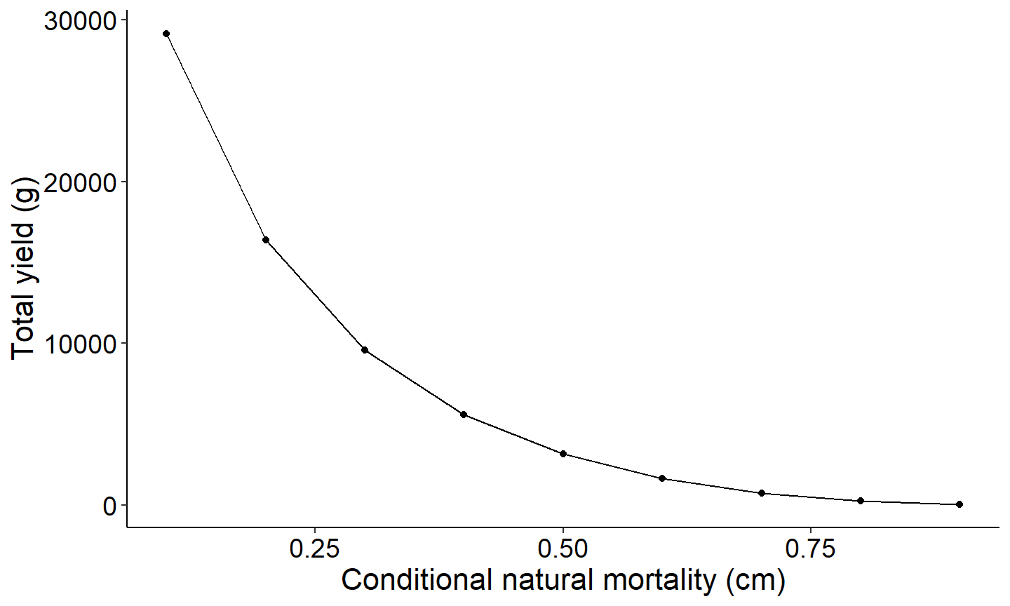

Number of fish that reach a specified size as a function of conditional natural mortality

The next figure demonstrates how to explore the number of fish reaching a specified length. This figure creates a plot showing the number of fish reaching 350mm as a function of conditional natural mortality.

#Plot number of fish reaching 350 mm as a function of cm
ggplot(data=Res_1,mapping=aes(x=cm ,y=`nAt350`)) +
  geom_point() +
  geom_line() +
  labs(y="Number of fish at 450 mm",x="Conditional natural mortality (cm )") +
  theme_FAMS()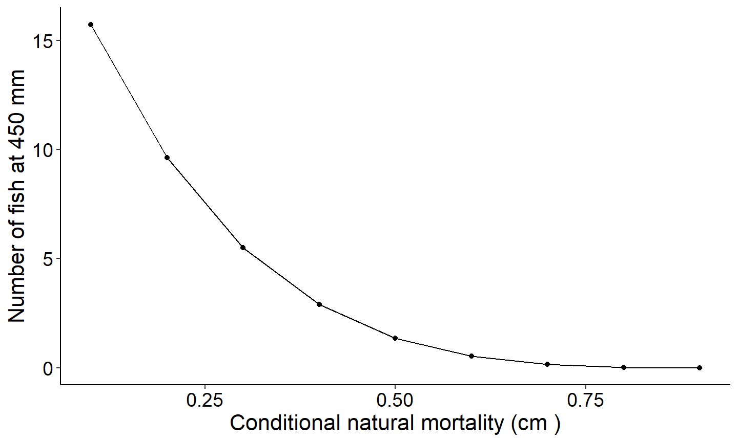

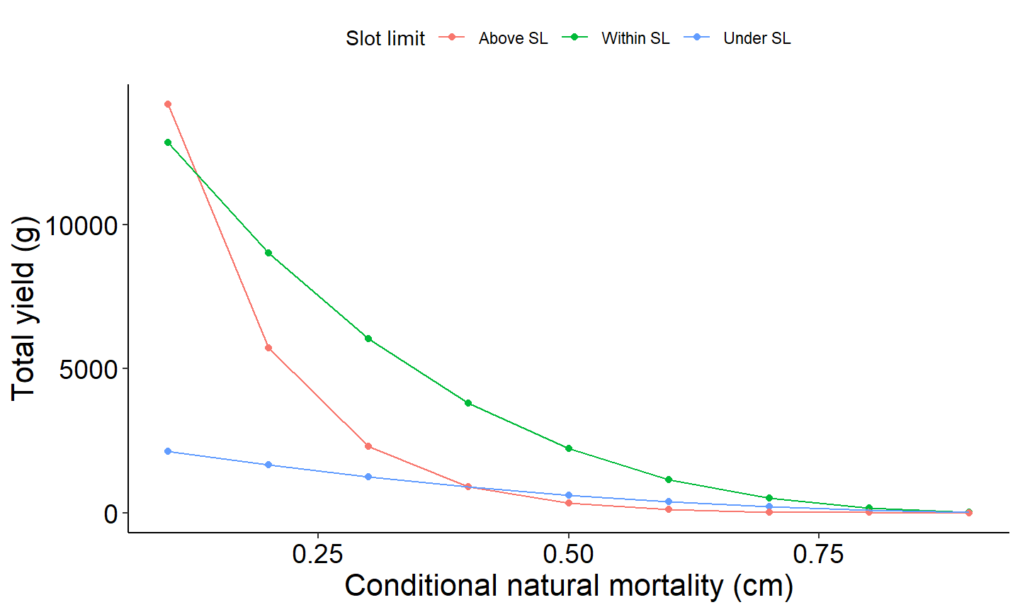
The last example figure plots yield as a function of conditional natural mortality across the three size classes; above slot limit, within slot limit, and above slot limit.

# Yield under, in, and above the slot limit vs Conditional Natural Mortality (cm)
# Select columns for plotting
plot_data <- Res_1 %>%
  select(cm, yieldUnder, yieldIn, yieldAbove) %>%
  pivot_longer(!cm, names_to="YieldCat",values_to="Yield")

# Generate plot
ggplot(data=plot_data,mapping=aes(x=cm,y=Yield,group=YieldCat,color=YieldCat)) +
  geom_point() +
  scale_color_discrete(name="Yield",labels=c("Above SL","Within SL","Under SL"))+
  geom_line() +
  labs(y="Total yield (g)",x="Conditional natural mortality (cm)") +
  theme_FAMS() +
  theme(legend.position = "top")+
  guides(color=guide_legend(title="Slot limit"))