Simulate a population using the dynamic pool model • rFAMS

library(rFAMS)
library(ggplot2)  ## to make figures
library(dplyr)    ## for filter

The objective of this article is to demonstrate how to use rFAMS to simulate a population and estimate population characteristics using the dynamic pool model. The dynamic pool model projects a population forward based on recruitment, life history parameters, and mortality. The dpmBH_minLL_fixed() function requires the following arguments:

simyears: A single numeric for the lower limit of minimum length limit for harvest in mm.
minLL:A single numeric representing the minimum length limit for harvest in mm.
cf: A matrix of conditional fishing mortality where each row represents a year and each column represents age. Ages are age-0 through maximum age.
cm: A matrix of conditional natural mortality where each row represents a year and each column represents age. Ages are age-0 through maximum age.
rec: A numeric vector of length simyears to specify recruitment each year. The vector can be geneated using the genRecruits() function.
lhparms: A named vector or list that contains values for each N0, tmax, Linf, K, t0, LWalpha, and LWbeta. See makeLH for definitions of these life history parameters. Also see details.
matchRicker: A logical that indicates whether the yield function should match that in Ricker (). Defaults to TRUE. The only reason to changed to FALSE is to try to match output from FAMS. See the YPR_FAMSvRICKER article.
species: is a single character to specify the species used in the simulation and will define the length for stock, quality, preferred, memorable, and trophy. Length categories are obtained from the FSA package, see the PSDlit documentation.
group: is a single character to specify the sub-group name of a species used in the simulation and will define the length for stock, quality, preferred, memorable, and trophy. Length categories are obtained from the FSA package, see the PSDlit documentation.

Organize input parameters

simyears and minLL require a single numeric value. This example simulates a population for 50 years with a minimum length limit of 400mm.

simyears <- 50
minLL <- 400

The lhparms requires a list or vector that is created with the makeLH() function. The makeLH() function creates a list of the life history parameters needed. Including, the initial number of recruits, maximum age of fish in your population, von Bertalanffy growth model parameters ( $L_\infty$ , $K$ , and $t_0$ ), and parameters from the log10-transformed weight length model (alpha and beta). By default, the makeLH() returns a list. Growth length-weight model paramaters can be generated from functions in the FSA package. See the Make Life History object article for more details. The example below uses the following life history parameters:

# create life history parameter object
LH <- makeLH(N0=100,tmax=15,Linf=1349.5,K=0.111,t0=0.065,LWalpha=-5.2147,LWbeta=3.153)

cf and cm are a matrix with rows = simyears (number of years specified in the simulation) and columns = tmax (maximum age). This example assigns a cm of 0 to the first year and 0.18 to the remaining years and is constant across ages; and a cf of 0 for the first year and 0.33 to the remaining years and is constant across ages. Note, Ages must be age-0 through maximum age. Thus, a cf and cm matrix will have maximum age plus on one rows.

cm <- matrix(rep(c(rep(0,1), rep(0.18,(LH$tmax))), simyears),nrow=simyears,byrow=TRUE)
cf <- matrix(rep(c(rep(0,1), rep(0.33,(LH$tmax))), simyears),nrow=simyears,byrow=TRUE)

Recruitment must be a vector of length simyears and contain a single value for each year. Users can specify the vector manually or use the genRecruits() function which allows the user to specify different trends in recruitment. This example sets recruitment to a fixed 1000 individuals each year.

rec <- genRecruits(method = "fixed", nR = 1000, simyears = simyears)

Run the dynamic pool model

The dpmBH_minLL_fixed function will use all the arguments above to simulate the population and generate a list with two data.frame object. The first list item contains a data.frame with a summary by age and the second list item contains a data.frame with a summary by year. The example used here specifies “Striped Bass” that are in the group “landlocked”. The species and group are used to assign appropriate PSD categories see FSA package for more information about PSD categories.

#run dynamic pool simulations
out1<-dpmBH_minLL_fixed(simyears = simyears, minLL = minLL, cf = cf, cm = cm, rec = rec, lhparms = LH,
           matchRicker=FALSE,species="Striped Bass",group="landlocked")

View the first few lines of each summary

head(out1[[1]])  #Summary by age
#>   year yc age   length     weight    nstart exploitation expect_nat_death   cf
#> 1    1  1   0   0.0000    0.00000 1000.0000    0.0000000        0.0000000 0.00
#> 2    2  1   1 133.0349   30.35037 1000.0000    0.0000000        0.1800000 0.33
#> 3    3  1   2 260.8383  253.58225  820.0000    0.0000000        0.1800000 0.33
#> 4    4  1   3 375.2145  798.00101  672.4000    0.3012967        0.1493033 0.33
#> 5    5  1   4 477.5741 1707.32249  405.4091    0.3012967        0.1493033 0.33
#> 6    6  1   5 569.1797 2968.94019  222.7318    0.3012967        0.1493033 0.33
#>     cm         F         M         Z      S   biomass  nharvest      ndie
#> 1 0.00 0.0000000 0.0000000 0.0000000 1.0000      0.00   0.00000   0.00000
#> 2 0.18 0.0000000 0.1984509 0.1984509 0.8200  30350.37   0.00000 180.00000
#> 3 0.18 0.0000000 0.1984509 0.1984509 0.8200 207937.44   0.00000 147.60000
#> 4 0.18 0.4004776 0.1984509 0.5989285 0.5494 536575.88 158.28150 108.70941
#> 5 0.18 0.4004776 0.1984509 0.5989285 0.5494 692164.07 122.14843  60.52891
#> 6 0.18 0.4004776 0.1984509 0.5989285 0.5494 661277.27  67.10835  33.25458
#>      yield minLL   N0   Linf     K    t0 LWalpha LWbeta tmax notes
#> 1      0.0   400 1000 1349.5 0.111 0.065 -5.2147  3.153   15      
#> 2      0.0   400 1000 1349.5 0.111 0.065 -5.2147  3.153   15      
#> 3      0.0   400 1000 1349.5 0.111 0.065 -5.2147  3.153   15      
#> 4 205139.2   400 1000 1349.5 0.111 0.065 -5.2147  3.153   15      
#> 5 274569.3   400 1000 1349.5 0.111 0.065 -5.2147  3.153   15      
#> 6 245109.6   400 1000 1349.5 0.111 0.065 -5.2147  3.153   15
head(out1[[2]])  #Summary by year
#> # A tibble: 6 × 16
#>    year age_1plus Yield_age_1plus Total_biomass nharvest_age_1plus
#>   <int>     <dbl>           <dbl>         <dbl>              <dbl>
#> 1     2     1000               0         30350.                 0 
#> 2     3     1820               0        238288.                 0 
#> 3     4     2492.         205139.       774864.               158.
#> 4     5     2898.         479709.      1467028.               280.
#> 5     6     3121.         724818.      2128305.               348.
#> 6     7     3243.         921629.      2683609.               384.
#> # ℹ 11 more variables: ndie_age_1plus <dbl>, memorable <int>, preferred <int>,
#> #   quality <int>, stock <int>, substock <int>, trophy <dbl>, PSD <dbl>,
#> #   PSD_P <dbl>, PSD_M <dbl>, PSD_T <dbl>

Plot Results

The output contains a lot of information and there are several potential figures that can be constructed. Below are examples of a few figures that might be of interest. The first set of figures will explore the data summarized by age and the second set of figures will explore the data summarized by year. First, a custom theme is created to use across all plots.

# Custom theme for plots (to make look nice)
theme_FAMS <- function(...) {
 theme_bw() +
 theme(
   panel.grid.major=element_blank(),panel.grid.minor=element_blank(),
   axis.text=element_text(size=14,color="black"),
   axis.title=element_text(size=16,color="black"),
   axis.title.y=element_text(angle=90),
   axis.line=element_line(color="black"),
   panel.border=element_blank()
 )
}

Exploring the summary by age output

The three figures below plot 1) yield vs age of a single year class 2) harvest vs age and 3) biomass vs age. Note since recruitment, cf, and cm was fixed across all year classes, all year classes will have the same age vs total yield.

#Plot date using summary by age for a specific year class
#filter for year class = 40
plotdat<- out1[[1]] |> filter(yc==40)

#Plot yield vs age
ggplot(data=plotdat,mapping=aes(x=age,y=yield)) +
  geom_point() +
  geom_line() +
  labs(y="Total yield (g)",x="Age") +
  theme_FAMS()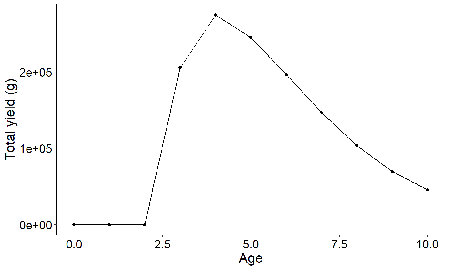


#Plot Number harvested vs age
ggplot(data=plotdat,mapping=aes(x=age,y=nharvest)) +
  geom_point() +
  geom_line() +
  labs(y="Number harvested",x="Age") +
  theme_FAMS()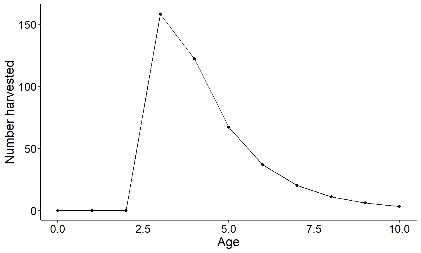


#Plot Number biomass vs age
ggplot(data=plotdat,mapping=aes(x=age,y=biomass)) +
  geom_point() +
  geom_line() +
  labs(y="Biomass (g)",x="Age") +
  theme_FAMS()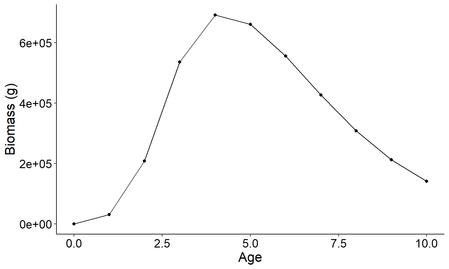

Exploring the summary by year output

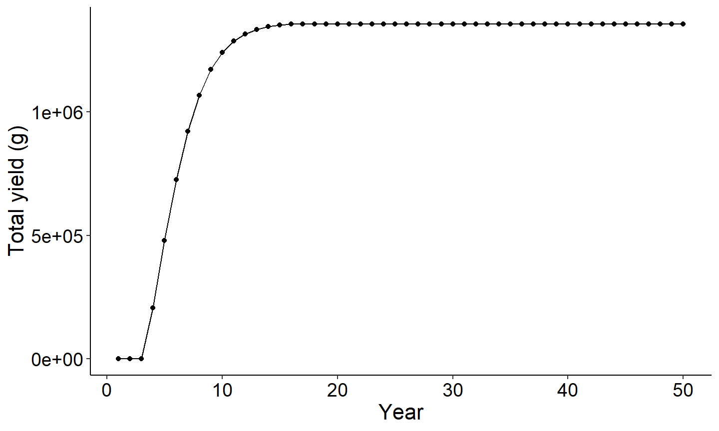
The next set of figures will explore the output summary by year. The first figure is PSD vs year and the second figure is Yield of age 1 plus vs year. Note each figure reaches an asymtote once all age classes are present in the population. This is because recruitment, cm, and cf are held constant across years.

#Use summary by year data frame to plot PSD vs year
ggplot(data=out1[[2]],mapping=aes(x=year,y=PSD)) +
  geom_point() +
  geom_line() +
  labs(y="PSD",x="Year") +
  theme_FAMS()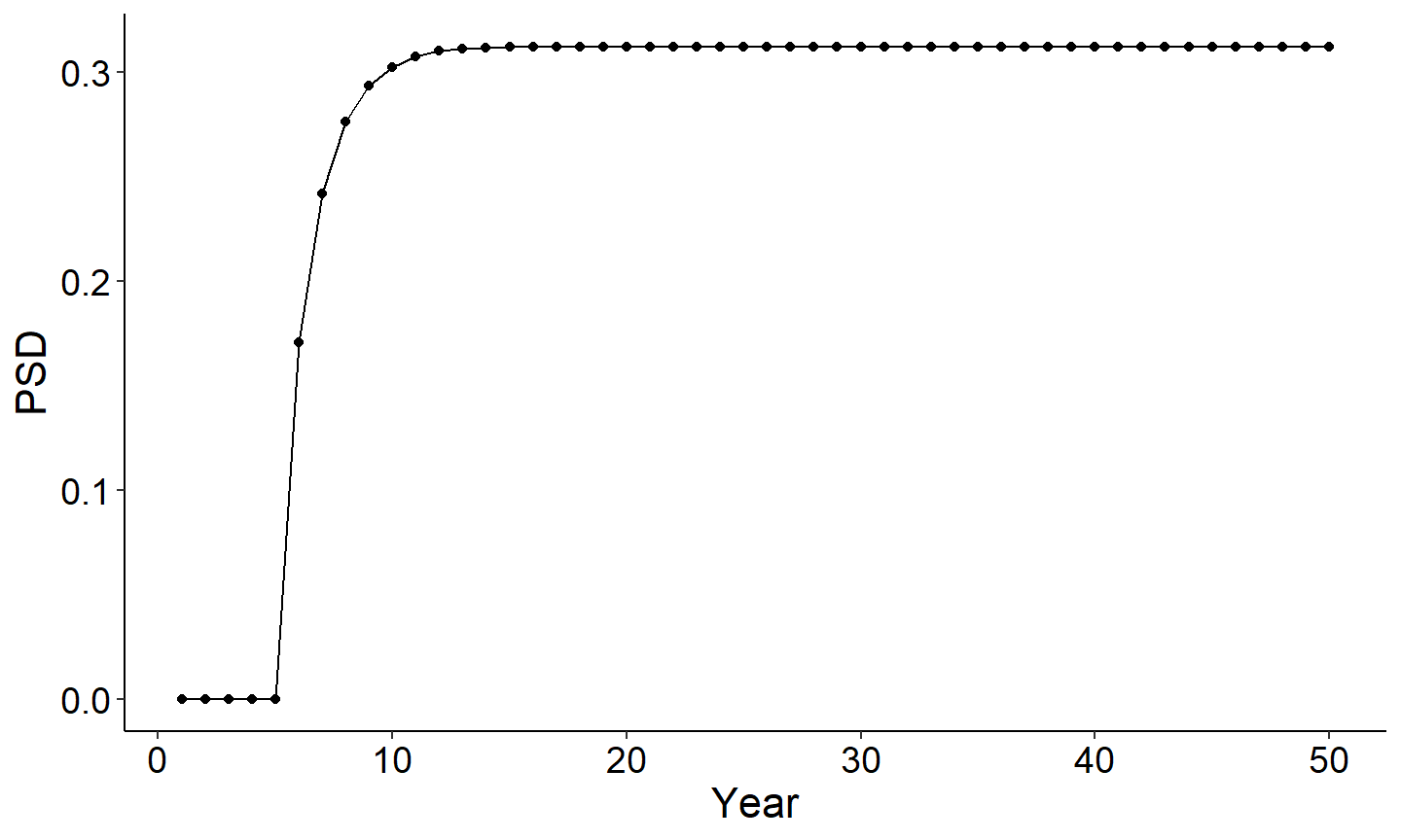


#Use summary by year data frame to plot yield vs year
ggplot(data=out1[[2]],mapping=aes(x=year,y=Yield_age_1plus)) +
  geom_point() +
  geom_line() +
  labs(y="Total yield (g)",x="Year") +
  theme_FAMS()