The objective of this article is to demonstrate how to use rFAMS to calculate yield based on a protective slot length limit with multiple values of conditional natural mortality. Separate conditional fishing mortality for fish below slot, within slot, and above slot must be specified. This allows the user to investigate a protective slot where fish are protected from harvest within a length range (i.e., conditional fishing mortality within cfIn = 0) and an inverted slot where small fish below the slot and large fish over the slot limit are protected while harvesting is allowed within the slot limit (i.e., conditional fishing mortality below cfBelow = 0, conditional fishing moratlity in cfIn = desired level of fishing mortality, and conditional fishing mortality above cfAbove = 0).
Build a life history parameter list
The first step for using any of the rFAMS simulation models is to create an object with life history parameters using the makeLH() function. The makeLH() function creates a list of the life history parameters needed. Including, the initial number of recruits, maximum age of fish in your population, von Bertalanffy growth model parameters (, , and ), and parameters from the log10-transformed weight length model (alpha and beta). By default, the makeLH() returns a list. Growth length-weight model paramaters can be generated from functions in the FSA package. The example below uses the following life history parameters:
- NO is the initial number of recruits, set to 100.
- tmax is the maximum age in the population in years, set to 15.
- Linf is the point estimate of asymptotic mean length from the von Bertalanffy growth model, set to 592mm.
- K (upper case) is the point estimate of the Brody growth coefficient from the von Bertalanffy growth model, set to 0.20.
- t0 is the point estimate of the x-intercept (i.e., theoretical age at a mean length of 0) from the von Bertalanffy growth model, set to -0.3.
- LWalpha is the point estimate of alpha from the length-weight regression on the log10 scale, set to -5.528.
- LWbeta is the point estimate of beta from the length-weight regression on the log10 scale, set to 3.273.
# create life history parameter object
LH <- makeLH(N0=100,tmax=15,Linf=592,K=0.20,t0=-0.3,LWalpha=-5.528,LWbeta=3.273)
Estimate yield for one minimum length limit and variable conditional fishing and conditional natural mortality.
The function yprBH_SlotLL() function is used when yield is estimated with a slot limit and conditional fishing mortality is specified below, within, and above the slot. This function requires a recruitment length recruitmentTL (i.e., the length where fish are susceptible to harvest, this is NOT the lower slot limit); lower slot limit lowerSL; upper slot limit upperSL; conditional fishing mortality below the slot limit but above recruitment length cfBelow; conditional fishing mortality within the slot limit cfIn; conditional fishing mortality above the slot limit cfAbove; specified conditional natural mortality cm by supplying a vector of one or more conditional natural mortality values; set any length of interest to monitor loi; and the life history parameters lhparams.
rFAMS includes a function est_natmort() to estimate instantaneous natural mortality (M) and conditional natural mortality (cm) using parameters specified in the life history parameter object. See the FSA package for other methods of calculating M and cm. To generate the range and average M and cm using rFAMS:
est_natmort(LH, incl.avg = TRUE)
#>            method         M         cm                  givens
#> 1       HoenigNLS 0.4100226 0.33636478                 tmax=15
#> 2         HoenigO 0.2954353 0.25579246                 tmax=15
#> 3        HoenigO2 0.2963197 0.25645032                 tmax=15
#> 4        HoenigLM 0.3612696 0.30320890                 tmax=15
#> 5    HewittHoenig 0.2813333 0.24522330                 tmax=15
#> 6           tmax1 0.3406000 0.28865661                 tmax=15
#> 7       PaulyLNoT 0.3308050 0.28165477        K=0.2, Linf=59.2
#> 8              K1 0.3384000 0.28708993                   K=0.2
#> 9              K2 0.4080000 0.33502112                   K=0.2
#> 10      HamelCope 0.3600000 0.30232367                 tmax=15
#> 11       JensenK1 0.3000000 0.25918178                   K=0.2
#> 12       JensenK2 0.5040000 0.39589062                   K=0.2
#> 13 AlversonCarney 0.2821182 0.24581544          tmax=15, K=0.2
#> 14   ChenWatanabe 0.1018740 0.09685666 tmax=15, K=0.2, t0=-0.3
#> 15        AVERAGE 0.3292984 0.27782360
To estimate yield with a slot limit the user must specify the lower slot limit lowerSL, upper slot limit upperSL, and optional recruitment length limit recruitmentTL which is the minimum length fish could be harvested at if harvest is allowed below the slot limit. The user must also specify conditional fishing mortality below, within, and above the slot. Specifying cf is where the user will determine if the slot limit is a protective slot (set cfIn = 0) with harvest below and above the slot, or an inverse slot (set cfBelow and cfAbove = 0) with harvest within the slot. In the example below, there is a protective slot and cm values range from 0.1 to 0.9 in increments of 0.1. It also monitors lengths of 200, 250, 300, and 350mm. FInally, there is an optional string to label the simulation.
# conditional natural mortality vector
cm <- seq(from = 0.1, to = 0.9, by = 0.1)
# length of interest vector
loi <- c(200,250,300,325,350)

Res_1 <- yprBH_SlotLL(lowerSL=250,upperSL=325,          # Set slot limit length
                      cfBelow=0.45,cfIn=0,cfAbove=0.25, # Set cf below, in, and above slot limit
                      cm=cm,                  # vector of cm
                      lhparms=LH,             # Specifies life history parameters
                      recruitmentTL=200,      # Set recruitment length
                      loi=loi,                # vector of lengths of interest
                      label="250 to 325")     # string to label simulation
The output object will be a data.frame with the following calculated values:
- cm A numeric representing conditional natural mortality
- yieldTotal is the calculated total yield
- nharvTotal is the calculated total number of harvested fish
- ndieTotal is the calculated total number of fish that die of natural death
- yieldBelow is the calculated yield below the slot limit
- yieldIn is the calculated yield within the slot limit
- yieldAbove is the calculated yield above the slot limit
- exploitationBelow is the exploitation rate below the slot limit
- exploitationIn is the exploitation rate within the slot limit
- exploitationAbove is the exploitation rate above the slot limit
- nharvestBelow is the number of harvested fish below the slot limit
- nharvestIn is the number of harvested fish within the slot limit
- nharvestAbove is the number of harvested fish above the slot limit
- n0die is the number of fish that die of natural death before entering the fishery at a minimum length
- ndieBelow is the number of fish that die of natural death below the slot limit
- ndieIn is the number of fish that die of natural deaths within the slot limit
- ndieAbove is the number of fish that die of natural deaths above the slot limit
- avglenBelow is the average length of fish harvested below the slot limit
- avglenIn is the average length of fish harvested within the slot limit
- avglenAbove is the average length of fish harvested above the slot limit
- avgwtBelow is the average weight of fish harvested below the slot limit
- avgwtIn is the average weight of fish harvested within the slot limit
- avgwtAbove is the average weight of fish harvested above the slot limit
- trBelow is the time for a fish to recruit to a minimum length limit (i.e., time to enter fishery)
- trIn is the time for a fish to recruit to a lower length limit of the slot limit
- trOver is the time for a fish to recruit to a upper length limit of the slot limit
- nrBelow is the number of fish at time trBelow (time they become harvestable size below the slot limit)
- nrIn is the number of fish at time trIn (time they reach the lower slot limit size)
- nrAbove is the number of fish at time trAbove (time they reach the upper slot limit size)
- FBelow is the estimated instantaneous rate of fishing mortality below the slot limit
- FIn is the estimated instantaneous rate of fishing mortality within the slot limit
- FAbove is the estimated instantaneous rate of fishing mortality above the slot limit
- MBelow is the estimated instantaneous rate of natural mortality below the slot limit
- MIn is the estimated instantaneous rate of natural mortality within the slot limit
- MAbove is the estimated instantaneous rate of natural mortality above the slot limit
- ZBelow is the estimated instantaneous rate of total mortality below the slot limit
- ZIn is the estimated instantaneous rate of total mortality within the slot limit
- ZAbove is the estimated instantaneous rate of total mortality above the slot limit
- SBelow is the estimated total survival below the slot limit
- SIn is the estimated total survival within the slot limit
- SAbove is the estimated total survival above the slot limit
- cfBelow A numeric representing conditional fishing mortality
- cfIn A numeric representing conditional fishing mortality
- cfOver A numeric representing conditional fishing mortality
- recruitmentTL A numeric representing the minimum length limit for recruiting to the fishery in mm.
- lowerSL A numeric representing the length of the lower slot limit in mm.
- upperSL A numeric representing the length of the upper slot limit in mm.
- nAtxxx is the number that reach the length of interest supplied. There will be one column for each length of interest.
For convenience the data.frame also contains the model input values (cf derived from cfBelow, cfIn, and cfOver; recruitmentTL; lowerSL; upperSL; cm derived from cmmin, cmmax, and cminc; N0; Linf; K; t0; LWalpha; LWbeta; and tmax).
View the first few rows of the output
head(Res_1)
#>   yieldTotal yieldBelow yieldIn yieldAbove nharvTotal ndieTotal nharvestBelow
#> 1  42308.228  3964.9645       0 38343.2634  59.552529  22.98342     26.910336
#> 2  20226.339  3091.0064       0 17135.3322  37.501897  29.91042     21.080642
#> 3   9822.674  2332.2837       0  7490.3901  23.975727  29.36807     15.993708
#> 4   4809.573  1686.3402       0  3123.2330  15.291391  25.37745     11.637517
#> 5   2347.811  1150.4916       0  1197.3190   9.519571  19.98013      7.999040
#> 6   1120.509   721.7631       0   398.7459   5.608765  14.30432      5.063981
#>   nharvestIn nharvestAbove    n0die ndieBelow   ndieIn ndieAbove  nrBelow
#> 1          0    32.6421933 16.93639  4.742575 6.285991 11.954858 83.06361
#> 2          0    16.4212547 32.49751  7.868381 9.304722 12.737315 67.50249
#> 3          0     7.9820193 46.64404  9.541990 9.929784  9.896294 53.35596
#> 4          0     3.6538739 59.32995  9.943750 8.945661  6.488039 40.67005
#> 5          0     1.5205306 70.50022  9.274288 7.042243  3.663598 29.49978
#> 6          0     0.5447837 80.08692  7.761445 4.807692  1.735180 19.91308
#>        nrIn   nrAbove  trBelow     trIn  trOver avglenBelow avglenIn
#> 1 51.410701 45.124710 1.761224 2.443479 3.68129    224.6247        0
#> 2 38.553462 29.248740 1.761224 2.443479 3.68129    224.2924        0
#> 3 27.820264 17.890480 1.761224 2.443479 3.68129    223.9166        0
#> 4 19.088779 10.143117 1.761224 2.443479 3.68129    223.4842        0
#> 5 12.226450  5.184207 1.761224 2.443479 3.68129    222.9755        0
#> 6  7.087658  2.279967 1.761224 2.443479 3.68129    222.3578        0
#>   avglenAbove avgwtBelow avgwtIn avgwtAbove   nAt200    nAt250    nAt300
#> 1    423.5651   147.3398       0  1174.6534 83.06361 51.410701 47.303370
#> 2    408.5157   146.6277       0  1043.4850 67.50249 38.553462 32.320412
#> 3    395.4809   145.8251       0   938.4079 53.35596 27.820264 20.986722
#> 4    384.3607   144.9055       0   854.7731 40.67005 19.088779 12.748365
#> 5    374.8445   143.8287       0   787.4350 29.49978 12.226450  7.069700
#> 6    366.5665   142.5288       0   731.9345 19.91308  7.087658  3.435713
#>      nAt325    nAt350  cm  expBelow expIn  expAbove   FBelow FIn    FAbove
#> 1 45.124710 37.196999 0.1 0.4293355     0 0.2378792 0.597837   0 0.2876821
#> 2 29.248740 22.753928 0.2 0.4077913     0 0.2252683 0.597837   0 0.2876821
#> 3 17.890480 13.033618 0.3 0.3851914     0 0.2120703 0.597837   0 0.2876821
#> 4 10.143117  6.850250 0.4 0.3612919     0 0.1981511 0.597837   0 0.2876821
#> 5  5.184207  3.201072 0.5 0.3357375     0 0.1833156 0.597837   0 0.2876821
#> 6  2.279967  1.261552 0.6 0.3079746     0 0.1672608 0.597837   0 0.2876821
#>      MBelow       MIn    MAbove    ZBelow       ZIn    ZAbove SBelow SIn SAbove
#> 1 0.1053605 0.1053605 0.1053605 0.7031975 0.1053605 0.3930426  0.495 0.9  0.675
#> 2 0.2231436 0.2231436 0.2231436 0.8209806 0.2231436 0.5108256  0.440 0.8  0.600
#> 3 0.3566749 0.3566749 0.3566749 0.9545119 0.3566749 0.6443570  0.385 0.7  0.525
#> 4 0.5108256 0.5108256 0.5108256 1.1086626 0.5108256 0.7985077  0.330 0.6  0.450
#> 5 0.6931472 0.6931472 0.6931472 1.2909842 0.6931472 0.9808293  0.275 0.5  0.375
#> 6 0.9162907 0.9162907 0.9162907 1.5141277 0.9162907 1.2039728  0.220 0.4  0.300
#>   cfBelow cfIn cfOver recruitmentTL lowerSL upperSL  N0 Linf   K   t0 LWalpha
#> 1    0.45    0   0.25           200     250     325 100  592 0.2 -0.3  -5.528
#> 2    0.45    0   0.25           200     250     325 100  592 0.2 -0.3  -5.528
#> 3    0.45    0   0.25           200     250     325 100  592 0.2 -0.3  -5.528
#> 4    0.45    0   0.25           200     250     325 100  592 0.2 -0.3  -5.528
#> 5    0.45    0   0.25           200     250     325 100  592 0.2 -0.3  -5.528
#> 6    0.45    0   0.25           200     250     325 100  592 0.2 -0.3  -5.528
#>   LWbeta tmax      label
#> 1  3.273   15 250 to 325
#> 2  3.273   15 250 to 325
#> 3  3.273   15 250 to 325
#> 4  3.273   15 250 to 325
#> 5  3.273   15 250 to 325
#> 6  3.273   15 250 to 325
Plot results
We will now create a series of figures to aid in interpreting the output. First, a custom theme is created to use across all plots.
# Custom theme for plots (to make look nice)
theme_FAMS <- function(...) {
 theme_bw() +
 theme(
   panel.grid.major=element_blank(),panel.grid.minor=element_blank(),
   axis.text=element_text(size=14,color="black"),
   axis.title=element_text(size=16,color="black"),
   axis.title.y=element_text(angle=90),
   axis.line=element_line(color="black"),
   panel.border=element_blank()
 )
}
Yield as a function of conditional natural mortality
The first figure will be a yield curve that displays the relationship between yield as a function of conditional natural mortality.
# Total Yield vs Conditional Natural Mortality (cm)
ggplot(data=Res_1,mapping=aes(x=cm,y=yieldTotal)) +
  geom_point() +
  geom_line() +
  labs(y="Total yield (g)",x="Conditional natural mortality (cm)") +
  theme_FAMS()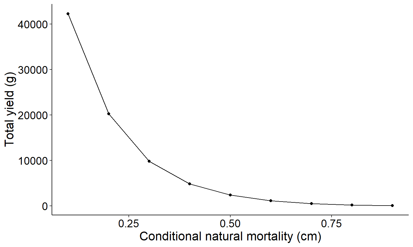
Number of fish that reach a specified size as a function of conditional natural mortality
The next figure demonstrates how to explore the number of fish reaching a specified length. This figure creates a plot showing the number of fish reaching 350mm as a function of conditional natural mortality.
#Plot number of fish reaching 350 mm as a function of cm
ggplot(data=Res_1,mapping=aes(x=cm ,y=`nAt350`)) +
  geom_point() +
  geom_line() +
  labs(y="Number of fish at 450 mm",x="Conditional natural mortality (cm )") +
  theme_FAMS()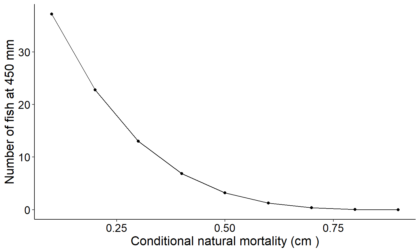
The last example figure plots yield as a function of conditional natural mortality across the three size classes; above slot limit, within slot limit, and above slot limit.
# Yield below, in, and above the slot limit vs Conditional Natural Mortality (cm)
# Select columns for plotting
plot_data <- Res_1 %>%
  select(cm, yieldBelow, yieldIn, yieldAbove) %>%
  pivot_longer(!cm, names_to="YieldCat",values_to="Yield")

# Generate plot
ggplot(data=plot_data,mapping=aes(x=cm,y=Yield,group=YieldCat,color=YieldCat)) +
  geom_point() +
  scale_color_discrete(name="Yield",labels=c("Above SL","Within SL","Below SL"))+
  geom_line() +
  labs(y="Total yield (g)",x="Conditional natural mortality (cm)") +
  theme_FAMS() +
  theme(legend.position = "top")+
  guides(color=guide_legend(title="Slot limit"))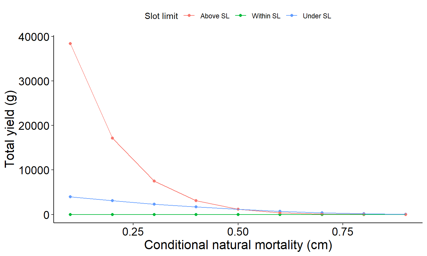
Compare yield across multiple slot limits
The label argument can be used to plot and compare results from multiple slot limits. The last example simulates yield below two additional slot limits and creates a single figure to compare yield across the three slot limits.
# Simulate yield using settings above with two additional slot limit ranges

Res_2 <- yprBH_SlotLL(lowerSL=325,upperSL=375,          # Set slot limit length
                      cfBelow=0.45,cfIn=0,cfAbove=0.25, # Set cf below, in, and above slot limit
                      cm=cm,                  # vector of cm
                      lhparms=LH,             # Specifies life history parameters
                      recruitmentTL=200,      # Set recruitment length
                      loi=loi,                # vector of lengths of interest
                      label="325 to 375")     # string to label simulation

Res_3 <- yprBH_SlotLL(lowerSL=375,upperSL=450,          # Set slot limit length
                      cfBelow=0.45,cfIn=0,cfAbove=0.25, # Set cf below, in, and above slot limit
                      cm=cm,                  # vector of cm
                      lhparms=LH,             # Specifies life history parameters
                      recruitmentTL=200,      # Set recruitment length
                      loi=loi,                # vector of lengths of interest
                      label="375 to 450")     # string to label simulation

Res_all <- rbind(Res_1,Res_2,Res_3)

ggplot(data=Res_all,mapping=aes(x=cm,y=yieldTotal,color=label)) +
    geom_line()+
    theme_FAMS() +
    theme(legend.position = "top")+
    guides(color=guide_legend(title="Slot limit"))