Estimate yield based on multiple minimum length limits • rFAMS

library(rFAMS)
library(ggplot2)  ## to make figures
library(tidyr)    ## for pivot_longer
library(dplyr)    ## for filter
library(metR)     ## geom_text_contour

The objective of this article is to demonstrate how to use rFAMS to calculate yield based on multiple minimum length limit with multiple values of conditional fishing and conditional natural mortality.

Build a life history parameter list

The first step for using any of the rFAMS simulation models is to create an object with life history parameters using the makeLH() function. THe makeLH() function creates a list of the life history parameters needed. Including, the initial number of recruits, maximum age of fish in your population, von Bertalanffy growth model parameters ( $L_\infty$ , $K$ , and $t_0$ ), and parameters from the log10-transformed weight length model (alpha and beta). By default, the makeLH() returns a list. Growth length-weight model paramaters can be generated from functions in the FSA package. The example below uses the following life history parameters: - NO is the initial number of recruits, set to 100. - tmax is the maximum age in the population in years, set to 15. - Linf is the point estimate of asymptotic mean length from the von Bertalanffy growth model, set to 592mm. - K (upper case) is the point estimate of the Brody growth coefficient from the von Bertalanffy growth model, set to 0.20. - t0 is the point estimate of the x-intercept (i.e., theoretical age at a mean length of 0) from the von Bertalanffy growth model, set to -0.3. - LWalpha is the point estimate of alpha from the length-weight regression on the log10 scale, set to -5.528. - LWbeta is the point estimate of beta from the length-weight regression on the log10 scale, set to 3.273.

# create life history parameter object
LH <- makeLH(N0=100,tmax=15,Linf=592,K=0.20,t0=-0.3,LWalpha=-5.528,LWbeta=3.273)

Estimate yield for multiple minimum length limit and multiple conditional fishing and conditional natural mortality.

The function yprBH_minLL_var() function is used when yield is estimated with a single fixed minimum length limit. This function requires the minimum length minLL; specified range of conditional fishing mortality by setting the minimum cfmin, maximum cfmax, and increment cfinc; specified range of conditional natural mortality by setting the minimum cmmin, maximum cmmax, and increment cminc; set any length of interest to monitor loi; and the life history parameters lhparams.

rFAMS includes a function est_natmort() to estimate instantaneous natural mortality (M) and conditional natural mortality (cm) using parameters specified in the life history parameter object. See the FSA package for other methods of calculating M and cm. To generate the range and average M and cm using rFAMS:

est_natmort(LH, incl.avg = TRUE)
#>            method         M         cm                  givens
#> 1       HoenigNLS 0.4100226 0.33636478                 tmax=15
#> 2         HoenigO 0.2954353 0.25579246                 tmax=15
#> 3        HoenigO2 0.2963197 0.25645032                 tmax=15
#> 4        HoenigLM 0.3612696 0.30320890                 tmax=15
#> 5    HewittHoenig 0.2813333 0.24522330                 tmax=15
#> 6           tmax1 0.3406000 0.28865661                 tmax=15
#> 7       PaulyLNoT 0.3308050 0.28165477        K=0.2, Linf=59.2
#> 8              K1 0.3384000 0.28708993                   K=0.2
#> 9              K2 0.4080000 0.33502112                   K=0.2
#> 10      HamelCope 0.3600000 0.30232367                 tmax=15
#> 11       JensenK1 0.3000000 0.25918178                   K=0.2
#> 12       JensenK2 0.5040000 0.39589062                   K=0.2
#> 13 AlversonCarney 0.2821182 0.24581544          tmax=15, K=0.2
#> 14   ChenWatanabe 0.1018740 0.09685666 tmax=15, K=0.2, t0=-0.3
#> 15        AVERAGE 0.3292984 0.27782360

Once you have decided the range of cf and cm and decided what minimum length limit to consider, you can now proceed to estimating yield. The following example uses the life history object created above with a minimum length limit of 200mm, cf from 0.1 to 0.9 with increments of 0.1, cm from 0.1 to 0.9 with increments of 0.1, monitors lengths of 200, 250, 300, and 350mm.

Res_1 <- yprBH_minLL_var(lengthmin=200,lengthmax=500,lengthinc=50, #creates minimum length limits
                         cfmin=0.1,cfmax=0.9,cfinc=0.1, #creates vector of cf values
                         cmmin=0.1,cmmax=0.9,cminc=0.1, #creates vector of cm values
                         loi=c(400, 450, 500, 550),     #sets lengths of interest to monitor
                         lhparms=LH)                    #Specifies life history parameters

The output object will be a data.frame with the following calculated values:

yield is the estimated yield (in g).
exploitation is the exploitation rate.
nharvest is the number of harvested fish.
ndie is the number of fish that die of natural deaths.
nt is the number of fish at time tr (time they become harvestable size).
avgwt is the average weight of fish harvested.
avglen is the average length of fish harvested.
tr is the time for a fish to recruit to a minimum length limit (i.e., time to enter fishery).
F is the instantaneous rate of fishing mortality.
M is the instantaneous rate of natural mortality.
Z is the instantaneous rate of total mortality.
S is the (total) annual rate of survival.
nAtxxx is the number that reach the length of interest supplied. There will be one column for each length of interest.

For convenience the data.frame also contains the model input values (minLL derived from lengthmin, lengthmax, and lengthinc; cf derived from cfmin, cfmax, and cfinc; cm derived from cmmin, cmmax, and cminc; N0; Linf; K; t0; LWalpha; LWbeta; and tmax).

View the first few rows of the output

head(Res_1)
#>      yield nharvest     ndie       nt       tr     avgwt   avglen   nAt400
#> 1 40818.31 41.53181 41.53181 83.06361 1.761224  982.8204 401.1080 39.15698
#> 2 42961.98 38.65116 38.65116 77.30232 2.443479 1111.5316 416.4771 42.07533
#> 3 44833.10 35.56322 35.56322 71.12644 3.233764 1260.6592 432.8090 45.72871
#> 4 45992.30 32.21300 32.21300 64.42599 4.172845 1427.7562 449.5853 50.48460
#> 5 45715.51 28.51544 28.51544 57.03087 5.330056 1603.1847 465.7891 57.03087
#> 6 42738.81 24.32552 24.32552 48.65103 6.838398 1756.9537 479.0075 57.03087
#>     nAt450   nAt500    nAt550 exploitation         F         M        Z    S
#> 1 28.49531 18.03716  7.895417        0.095 0.1053605 0.1053605 0.210721 0.81
#> 2 30.61904 19.38146  8.483857        0.095 0.1053605 0.1053605 0.210721 0.81
#> 3 33.27768 21.06435  9.220507        0.095 0.1053605 0.1053605 0.210721 0.81
#> 4 36.73864 23.25508 10.179461        0.095 0.1053605 0.1053605 0.210721 0.81
#> 5 41.50249 26.27054 11.499418        0.095 0.1053605 0.1053605 0.210721 0.81
#> 6 48.65103 30.79548 13.480121        0.095 0.1053605 0.1053605 0.210721 0.81
#>    cf  cm minLL  N0 Linf   K   t0 LWalpha LWbeta tmax notes
#> 1 0.1 0.1   200 100  592 0.2 -0.3  -5.528  3.273   15      
#> 2 0.1 0.1   250 100  592 0.2 -0.3  -5.528  3.273   15      
#> 3 0.1 0.1   300 100  592 0.2 -0.3  -5.528  3.273   15      
#> 4 0.1 0.1   350 100  592 0.2 -0.3  -5.528  3.273   15      
#> 5 0.1 0.1   400 100  592 0.2 -0.3  -5.528  3.273   15      
#> 6 0.1 0.1   450 100  592 0.2 -0.3  -5.528  3.273   15

Plot results

We will now create a series of figures to aid in interpreting the output. First, a custom theme is created to use across all plots.

# Custom theme for plots (to make look nice)
theme_FAMS <- function(...) {
 theme_bw() +
 theme(
   panel.grid.major=element_blank(),panel.grid.minor=element_blank(),
   axis.text=element_text(size=14,color="black"),
   axis.title=element_text(size=16,color="black"),
   axis.title.y=element_text(angle=90),
   axis.line=element_line(color="black"),
   panel.border=element_blank()
 )
}

Yield as a function of exploitation

The first graph will be a yield curve that displays the relationship between yield as a function of exploitation for a specified conditional natural morality cm. The example below uses cm = 0.30, which is close to the estimated mean cm above of 0.27

# Round cm to account for "floating point arithmetic inaccuracies"
# will be fixed in next version of rFAMS so this isn't needed
Res_1$cm <- round(Res_1$cm,8)

# Extract results for cm=0.40 and minimum length limit=400
plot_dat <- Res_1 |> dplyr::filter(cm==0.30,minLL==400)

ggplot(data=plot_dat,mapping=aes(x=exploitation,y=yield)) +
  geom_point() +
  geom_line() +
  labs(y="Total yield (g)",x="Exploitation (u)") +
  theme_FAMS()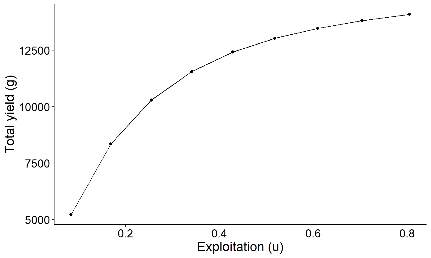

This next graph plots yield curves as a function of exploitation with multiple minimum lengths for a specified conditional natural morality cm. The example below uses cm = 0.30, as above.

# Round cm to account for "floating point arithmetic inaccuracies"
# will be fixed in next version of rFAMS so this isn't needed
Res_1$cm <- round(Res_1$cm,8)

# Extract results for cm=0.40 and minimum length limit=400
plot_dat <- Res_1 |> dplyr::filter(cm==0.30)

ggplot(data=plot_dat,mapping=aes(y=yield,x=exploitation,group=minLL,color=minLL)) +
  geom_line(linewidth=1) +
  scale_color_gradient2(high="black") +
  labs(y="Total yield (g)",x="Exploitation (u)",color="Min Length Limit") +
  theme_FAMS()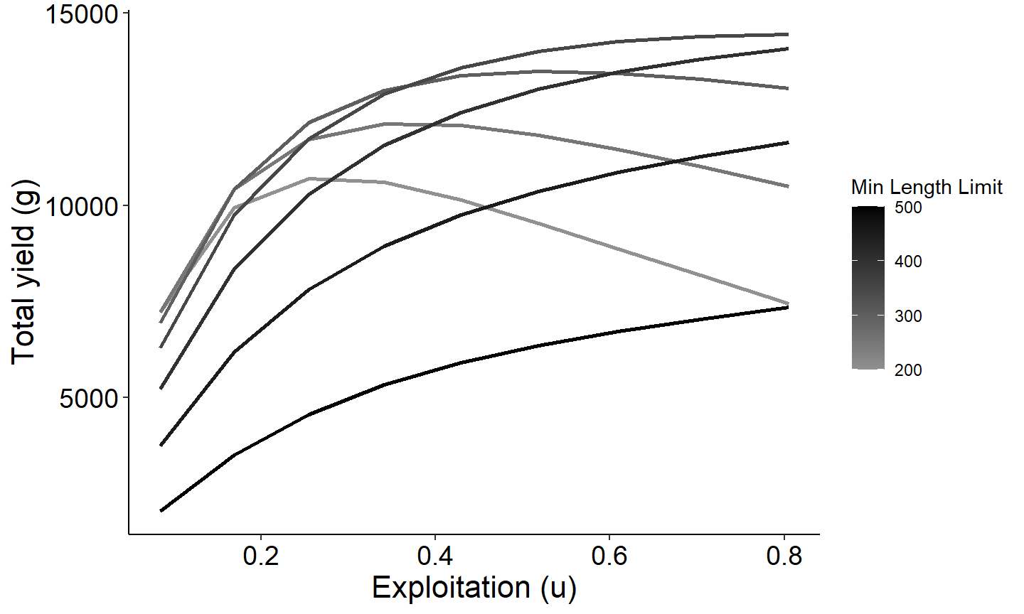

Number of fish that reach a specified size as a function of exploitation

The next graph demonstrates how to explore the number of fish reaching a specified length. This figure creates a plot showing the number of fish reaching 450mm as a function of exploitation. Note this is based on a conditional natural mortality cm of 0.30 which was filtered out in the code block above.

# Extract results for cm=0.40 and minimum length limit=400
plot_dat <- Res_1 |> dplyr::filter(cm==0.30,minLL==400)

ggplot(data=plot_dat,mapping=aes(x=exploitation,y=`nAt450`)) +
  geom_point() +
  geom_line() +
  labs(y="Number of fish at 450 mm",x="Exploitation (u)") +
  theme_FAMS()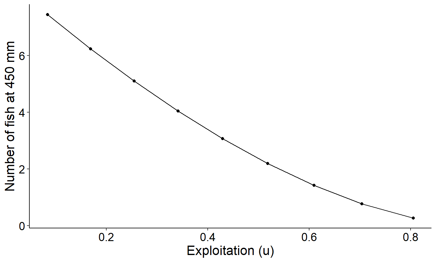

The next example graph plots the number of fish reaching all the lengths of interests we monitored as a function of exploitation with conditional natural mortality cm of 0.30 which was filtered out above.

# Select columns for plotting and convert to long
plot_data_long <- plot_dat %>%
 select(exploitation,`nAt400`, `nAt450`, `nAt500`, `nAt550`) %>%
 pivot_longer(!exploitation, names_to="loi",values_to="number")

# Generate plot
ggplot(data=plot_data_long,mapping=aes(x=exploitation,y=number,group=loi,color=loi)) +
 geom_point() +
 scale_color_discrete(name="Yield",labels=c("N at 400 mm", "N at 450 mm", "N at 500 mm", "N at 550 mm"))+
 geom_line() +
 labs(y="Number of fish",x="Exploitation (u)") +
 theme_FAMS() +
 theme(legend.position = "top")+
 guides(color=guide_legend(title="Length of interest"))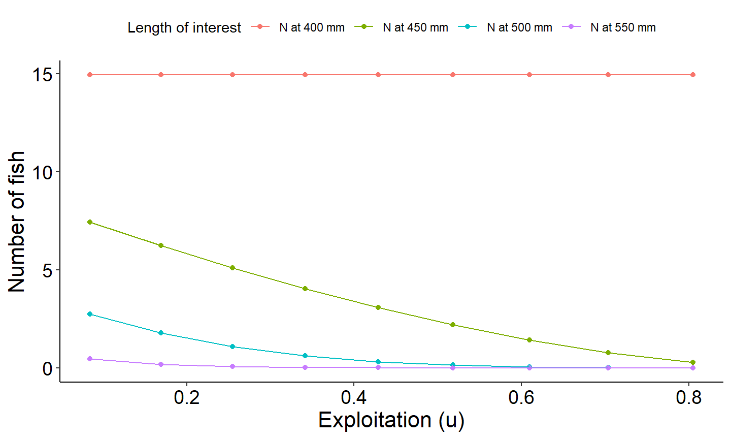

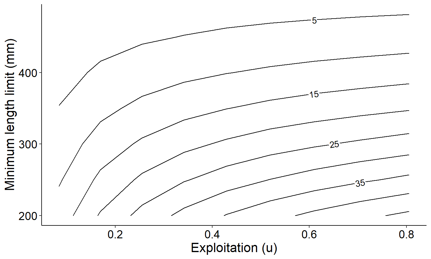
Isopleths of yield and number harvested

The final two graphs demonstrate how to construct isopleths using the ggplot2 and metR packages. We will use the same data from above that is filtered for a conditional natural mortality cm of 0.30.

# Extract results for cm=0.40 and minimum length limit=400
plot_dat <- Res_1 |> dplyr::filter(cm==0.30)

# Yield isopleths for varying minLL and exploitation with cm=0.40
# Using same data as previous example
ggplot(data=plot_dat,mapping=aes(x=exploitation,y=minLL,z=yield)) +
  geom_contour2(aes(label = after_stat(level))) +
  xlab("Exploitation (u)") +
  ylab("Minimum length limit (mm)") +
  theme_FAMS()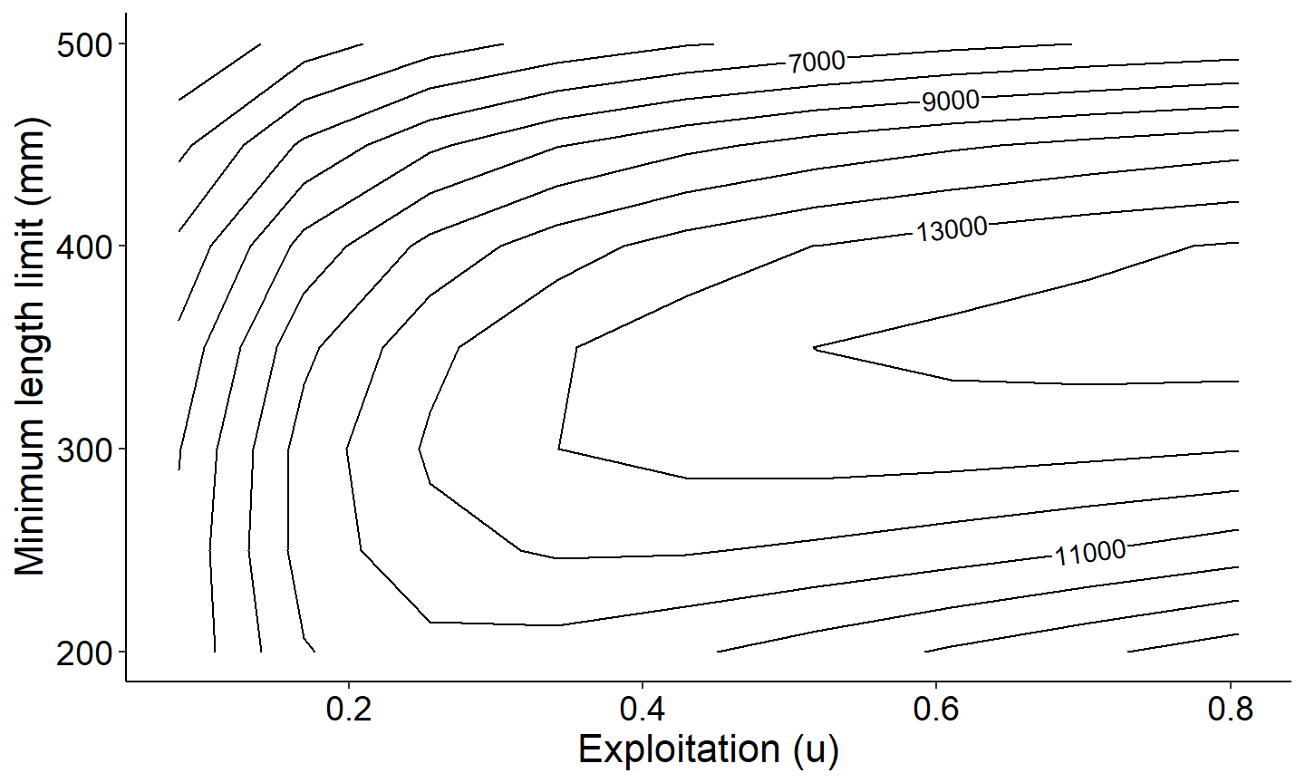


# Same isopleth as previous but using number harvested instead of yield
ggplot(data=plot_dat,mapping=aes(x=exploitation,y=minLL,z=nharvest)) +
  geom_contour2(aes(label = after_stat(level))) +
  xlab("Exploitation (u)")+
  ylab("Minimum length limit (mm)")+
  theme_FAMS()