Estimate yield based on a single minimum length limit • rFAMS

library(rFAMS)
library(ggplot2)  ## to make figures
library(tidyr)    ## for pivot_longer
library(dplyr)    ## for filter

The objective of this article is to demonstrate how to use rFAMS to calculate yield based on a fixed minimum length limit with multiple values of conditional fishing and conditional natural mortality.

Build a life history parameter list

The first step for using any of the rFAMS simulation models is to create an object with life history parameters using the makeLH() function. THe makeLH() function creates a list of the life history parameters needed. Including, the initial number of recruits, maximum age of fish in your population, von Bertalanffy growth model parameters ( $L_\infty$ , $K$ , and $t_0$ ), and parameters from the log10-transformed weight length model (alpha and beta). By default, the makeLH() returns a list. Growth length-weight model paramaters can be generated from functions in the FSA package. The example below uses the following life history parameters:

NO is the initial number of recruits, set to 100.
tmax is the maximum age in the population in years, set to 15.
Linf is the point estimate of asymptotic mean length from the von Bertalanffy growth model, set to 592mm.
K (upper case) is the point estimate of the Brody growth coefficient from the von Bertalanffy growth model, set to 0.20.
t0 is the point estimate of the x-intercept (i.e., theoretical age at a mean length of 0) from the von Bertalanffy growth model, set to -0.3.
LWalpha is the point estimate of alpha from the length-weight regression on the log10 scale, set to -5.528.
LWbeta is the point estimate of beta from the length-weight regression on the log10 scale, set to 3.273.

# create life history parameter object
LH <- makeLH(N0=100,tmax=15,Linf=592,K=0.20,t0=-0.3,LWalpha=-5.528,LWbeta=3.273)

Estimate yield for one minimum length limit and variable conditional fishing and conditional natural mortality.

The function yprBH_minLL_fixed() function is used when yield is estimated with a single fixed minimum length limit. This function requires the minimum length minLL; specified range of conditional fishing mortality by setting the minimum cfmin, maximum cfmax, and increment cfinc; specified range of conditional natural mortality by setting the minimum cmmin, maximum cmmax, and increment cminc; set any length of interest to monitor loi; and the life history parameters lhparams.

rFAMS includes a function est_natmort() to estimate instantaneous natural mortality (M) and conditional natural mortality (cm) using parameters specified in the life history parameter object. See the FSA package for other methods of calculating M and cm. To generate the range and average M and cm using rFAMS:

est_natmort(LH, incl.avg = TRUE)
#>            method         M         cm                  givens
#> 1       HoenigNLS 0.4100226 0.33636478                 tmax=15
#> 2         HoenigO 0.2954353 0.25579246                 tmax=15
#> 3        HoenigO2 0.2963197 0.25645032                 tmax=15
#> 4        HoenigLM 0.3612696 0.30320890                 tmax=15
#> 5    HewittHoenig 0.2813333 0.24522330                 tmax=15
#> 6           tmax1 0.3406000 0.28865661                 tmax=15
#> 7       PaulyLNoT 0.3308050 0.28165477        K=0.2, Linf=59.2
#> 8              K1 0.3384000 0.28708993                   K=0.2
#> 9              K2 0.4080000 0.33502112                   K=0.2
#> 10      HamelCope 0.3600000 0.30232367                 tmax=15
#> 11       JensenK1 0.3000000 0.25918178                   K=0.2
#> 12       JensenK2 0.5040000 0.39589062                   K=0.2
#> 13 AlversonCarney 0.2821182 0.24581544          tmax=15, K=0.2
#> 14   ChenWatanabe 0.1018740 0.09685666 tmax=15, K=0.2, t0=-0.3
#> 15        AVERAGE 0.3292984 0.27782360

Once you have decided the range of cf and cm and decided what minimum length limit to consider, you can now proceed to estimating yield. The following example uses the life history object created above with a minimum length limit of 200mm, cf from 0.1 to 0.9 with increments of 0.1, cm from 0.1 to 0.9 with increments of 0.1, monitors lengths of 200, 250, 300, and 350mm.

Res_1 <- yprBH_minLL_fixed(minLL=200,                     #Specifies minimum length limits
                          cfmin=0.1,cfmax=0.9,cfinc=0.1,  #creates vector of cf values
                          cmmin=0.1,cmmax=0.9,cminc=0.1,  #creates vector of cm values
                          loi=c(200,250,300,350),         #sets lengths of interest to monitor
                          lhparms=LH)                     #Specifies life history parameters

The output object will be a data.frame with the following calculated values:

yield is the estimated yield (in g).
exploitation is the exploitation rate.
nharvest is the number of harvested fish.
ndie is the number of fish that die of natural deaths.
nt is the number of fish at time tr (time they become harvestable size).
avgwt is the average weight of fish harvested.
avglen is the average length of fish harvested.
tr is the time for a fish to recruit to a minimum length limit (i.e., time to enter fishery).
F is the instantaneous rate of fishing mortality.
M is the instantaneous rate of natural mortality.
Z is the instantaneous rate of total mortality.
S is the (total) annual rate of survival.
Natxxx is the number that reach the length of interest supplied. There will be one column for each length of interest.

For convenience the data.frame also contains the model input values (minLL; cf derived from cfmin, cfmax, and cfinc; cm derived from cmmin, cmmax, and cminc; N0; Linf; K; t0; LWalpha; LWbeta; and tmax).

View the first few rows of the output

head(Res_1)
#>      yield nharvest      ndie       nt       tr    avgwt   avglen   nAt200
#> 1 40818.31 41.53181 41.531806 83.06361 1.761224 982.8204 401.1080 83.06361
#> 2 43838.62 56.42277 26.640842 83.06361 1.761224 776.9668 373.3149 83.06361
#> 3 38000.03 64.12215 18.941457 83.06361 1.761224 592.6194 343.6662 83.06361
#> 4 31527.25 68.86072 14.202892 83.06361 1.761224 457.8408 317.6133 83.06361
#> 5 26155.89 72.10364 10.959976 83.06361 1.761224 362.7542 295.8074 83.06361
#> 6 21929.40 74.49745  8.566157 83.06361 1.761224 294.3644 277.5167 83.06361
#>     nAt250   nAt300    nAt350 exploitation         F         M         Z    S
#> 1 71.94063 60.90477 49.970236    0.0950000 0.1053605 0.1053605 0.2107210 0.81
#> 2 66.38579 51.20675 37.614122    0.1901961 0.2231436 0.1053605 0.3285041 0.72
#> 3 60.60519 42.06605 27.258148    0.2856268 0.3566749 0.1053605 0.4620355 0.63
#> 4 54.55505 33.52354 18.795163    0.3813455 0.5108256 0.1053605 0.6161861 0.54
#> 5 48.17405 25.63022 12.108518    0.4774293 0.6931472 0.1053605 0.7985077 0.45
#> 6 41.37097 18.45221  7.069371    0.5739983 0.9162907 0.1053605 1.0216512 0.36
#>    cf  cm minLL  N0 Linf   K   t0 LWalpha LWbeta tmax notes
#> 1 0.1 0.1   200 100  592 0.2 -0.3  -5.528  3.273   15      
#> 2 0.2 0.1   200 100  592 0.2 -0.3  -5.528  3.273   15      
#> 3 0.3 0.1   200 100  592 0.2 -0.3  -5.528  3.273   15      
#> 4 0.4 0.1   200 100  592 0.2 -0.3  -5.528  3.273   15      
#> 5 0.5 0.1   200 100  592 0.2 -0.3  -5.528  3.273   15      
#> 6 0.6 0.1   200 100  592 0.2 -0.3  -5.528  3.273   15

Plot results

We will now create a series of figures to aid in interpreting the output. First, a custom theme is created to use across all plots.

# Custom theme for plots (to make look nice)
theme_FAMS <- function(...) {
 theme_bw() +
 theme(
   panel.grid.major=element_blank(),panel.grid.minor=element_blank(),
   axis.text=element_text(size=14,color="black"),
   axis.title=element_text(size=16,color="black"),
   axis.title.y=element_text(angle=90),
   axis.line=element_line(color="black"),
   panel.border=element_blank()
 )
}

Yield as a function of exploitation

The first figure will be a yield curve that displays the relationship between yield as a function of exploitation for a specified conditional natural morality cm. The example below uses cm = 0.30, which is close to the estimated mean cm above of 0.27.

# Round cm to account for "floating point arithmetic inaccuracies"
# will be fixed in next version of rFAMS so this isn't needed
Res_1$cm <- round(Res_1$cm,8)

# Extract results for cm=0.30
plot_dat <- Res_1 |> dplyr::filter(cm==0.30)

ggplot(data=plot_dat,mapping=aes(x=exploitation,y=yield)) +
 geom_point() +
 geom_line() +
 labs(y="Yield (g)",x="Exploitation (u)") +
 theme_FAMS()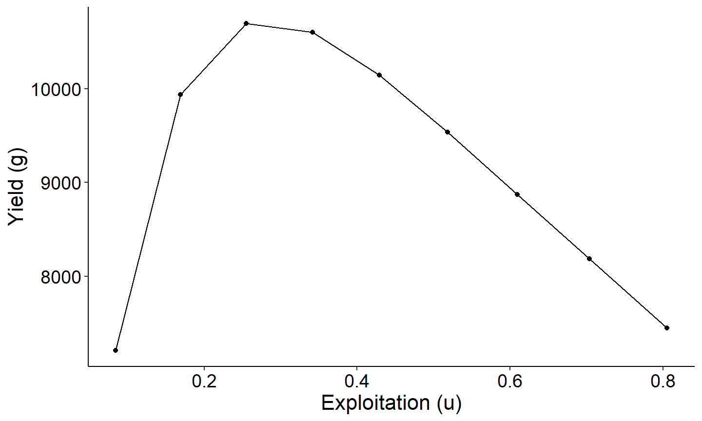

Number of fish that reach a specified size as a function of exploitation

The next figure demonstrates how to explore the number of fish reaching a specified length. This figure creates a plot showing the number of fish reaching 300mm as a function of exploitation. Note this is based on a conditional natural mortality cm of 0.30 which was filtered out in the code block above.

ggplot(data=plot_dat,mapping=aes(x=exploitation,y=`nAt300`)) +
 geom_point() +
 geom_line() +
 labs(y="Number of fish at 300 mm",x="Exploitation (u)") +
 theme_FAMS()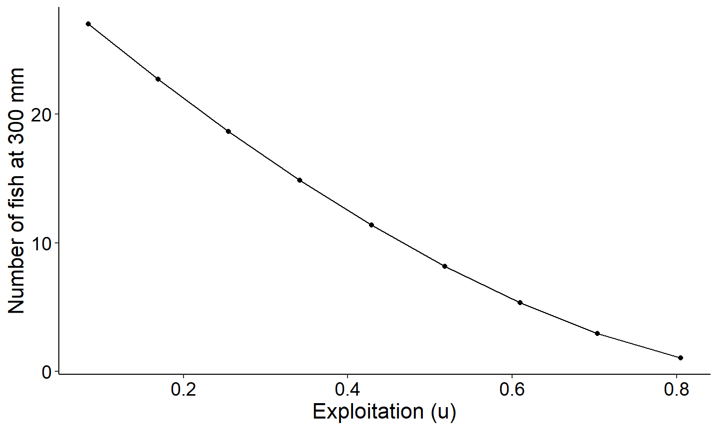

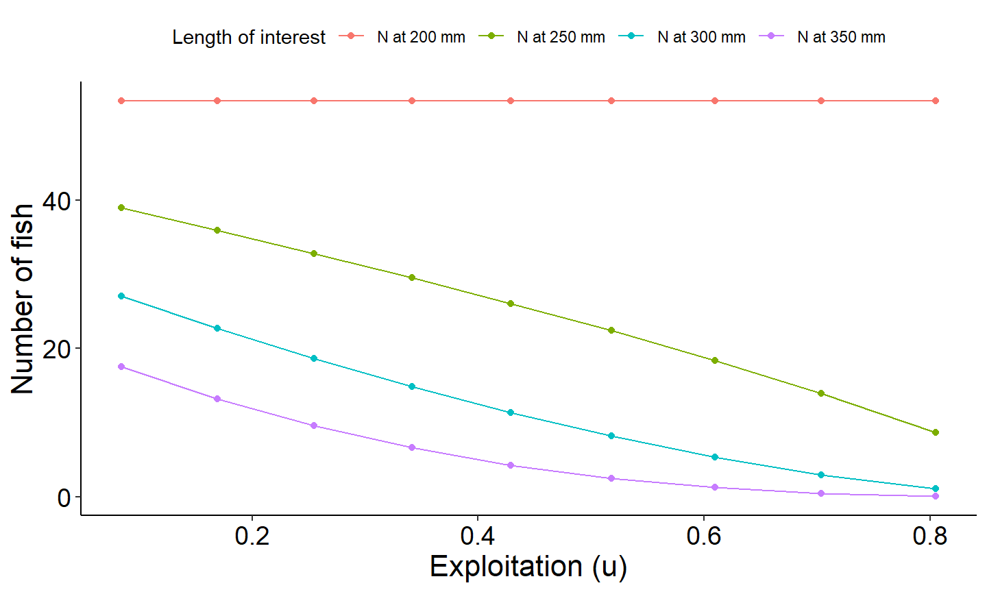
The last example figure plots the number of fish reaching all the lengths of interests we monitored as a function of exploitation with conditional natural mortality cm of 0.30 which was filtered out above.

# Select columns for plotting and convert to long
plot_data_long <- plot_dat %>%
 select(exploitation,`nAt200`, `nAt250`, `nAt300`, `nAt350`) %>%
 pivot_longer(!exploitation, names_to="loi",values_to="number")

# Generate plot
ggplot(data=plot_data_long,mapping=aes(x=exploitation,y=number,group=loi,color=loi)) +
 geom_point() +
 scale_color_discrete(name="Yield",labels=c("N at 200 mm", "N at 250 mm", "N at 300 mm", "N at 350 mm"))+
 geom_line() +
 labs(y="Number of fish",x="Exploitation (u)") +
 theme_FAMS() +
 theme(legend.position = "top")+
 guides(color=guide_legend(title="Length of interest"))