Main function to simulate expected yield using the Beverton-Holt Yield Per Recruit model for a slot limit

Main wrapper function to estimate yield using the Beverton-Holt YPR model. This main function accepts a range of values for cf, cm, recruitment length, lower slot limit length, and upper slot limit length.

Usage

yprBH_SlotLL(
  recruitmentTL,
  lowerSL,
  upperSL,
  cfunder,
  cfin,
  cfabove,
  cmmin,
  cmmax,
  cminc,
  loi = NULL,
  lhparms,
  matchRicker = FALSE
)

Arguments

recruitmentTL: A numeric representing the minimum length limit for recruiting to the fishery in mm.
lowerSL: A numeric representing the length of the lower slot limit in mm.
upperSL: A numeric representing the length of the upper slot limit in mm.
cfunder: Single value, conditional fishing mortality under the lower slot limit.
cfin: Single value, conditional fishing mortality within the lower and upper slot limit.
cfabove: Single value, conditional fishing mortality over the upper slot limit.
cmmin: Single value, minimum conditional natural mortality
cmmax: Single value, maximum conditional natural mortality
cminc: Single value, increment to cycle from minimum to maximum conditional natural mortality
loi: A numeric vector for lengths of interest. Used to determine number of fish that reach desired lengths.
lhparms: A named vector or list that contains values for each N0, tmax, Linf, K, t0, LWalpha, and LWbeta. See makeLH for definitions of these life history parameters. Also see details.
matchRicker: A logical that indicates whether the yield function should match that in Ricker (). Defaults to TRUE. The only reason to changed to FALSE is to try to match output from FAMS. See the "YPR_FAMSvRICKER" article.

Value

A data.frame with the following calculated values:

yieldTotal is the calculated total yield
yieldUnder is the calculated yield under the slot limit
yieldIn is the calculated yield within the slot limit
yieldAbove is the calculated yield above the slot limit
nharvTotal is the calculated total number of harvested fish
ndieTotal is the calculated total number of fish that die of natural death
nharvestUnder is the number of harvested fish under the slot limit
nharvestIn is the number of harvested fish within the slot limit
nharvestAbove is the number of harvested fish above the slot limit
n0die is the number of fish that die of natural death before entering the fishery at a minimum length
ndieUnder is the number of fish that die of natural death between entering the fishery and the lower slot limit
ndieIn is the number of fish that die of natural deaths within the slot limit
ndieAbove is the number of fish that die of natural deaths above the slot limit
nrUnder is the number of fish at time trUnder (time they become harvestable size under the slot limit)
nrIn is the number of fish at time trIn (time they reach the lower slot limit size)
nrAbove is the number of fish at time trAbove (time they reach the upper slot limit size)
trUnder is the time for a fish to recruit to a minimum length limit (i.e., time to enter fishery)
trIn is the time for a fish to recruit to a lower length limit of the slot limit
trOver is the time for a fish to recruit to a upper length limit of the slot limit
avglenUnder is the average length of fish harvested under the slot limit
avglenIn is the average length of fish harvested within the slot limit
avglenAbove is the average length of fish harvested above the slot limit
avgwtUnder is the average weight of fish harvested under the slot limit
avgwtIn is the average weight of fish harvested within the slot limit
avgwtAbove is the average weight of fish harvested above the slot limit
nAtxxx is the number that reach the length of interest supplied. There will be one column for each length of interest.
cm A numeric representing conditional natural mortality
expUnder is the exploitation rate under the slot limit
expIn is the exploitation rate within the slot limit
expAbove is the exploitation rate above the slot limit
FUnder is the estimated instantaneous rate of fishing mortality under the slot limit
FIn is the estimated instantaneous rate of fishing mortality within the slot limit
FAbove is the estimated instantaneous rate of fishing mortality above the slot limit
MUnder is the estimated instantaneous rate of natural mortality under the slot limit
MIn is the estimated instantaneous rate of natural mortality within the slot limit
MAbove is the estimated instantaneous rate of natural mortality above the slot limit
ZUnder is the estimated instantaneous rate of total mortality under the slot limit
ZIn is the estimated instantaneous rate of total mortality within the slot limit
ZAbove is the estimated instantaneous rate of total mortality above the slot limit
SUnder is the estimated total survival under the slot limit
SIn is the estimated total survival within the slot limit
SAbove is the estimated total survival above the slot limit
cfUnder A numeric representing conditional fishing mortality
cfIn A numeric representing conditional fishing mortality
cfOver A numeric representing conditional fishing mortality
recruitmentTL A numeric representing the minimum length limit for recruiting to the fishery in mm.
lowerSL A numeric representing the length of the lower slot limit in mm.
upperSL A numeric representing the length of the upper slot limit in mm.
N0 A numeric representing the initial number of new recruits entering the fishery OR a vector or list that contains named values for each N0, Linf, K, t0, LWalpha, LWbeta, and tmax
Linf A numeric representing the point estimate of the asymptotic mean length (L-infinity) from the von Bertalanffy growth model in mm
K A numeric representing the point estimate of the Brody growth coefficient from the von Bertalanffy growth model
t0 A numeric representing the point estimate of the x-intercept (i.e., theoretical age at a mean length of 0) from the von Bertalanffy growth model
LWalpha A numeric representing the point estimate of alpha from the length-weight regression on the log10 scale.
LWbeta A numeric representing the point estimate of beta from the length-weight regression on the log10 scale.
tmax An integer representing maximum age in the population in years

Details

Details will be filled out later

Author

Jason C. Doll, jason.doll@fmarion.edu

Examples

#Load other required packages for organizing output and plotting
library(ggplot2)  #for plotting
library(dplyr)    #for select
library(tidyr)    #for pivot_longer

# Life history parameters to be used below
LH <- makeLH(N0=100,tmax=15,Linf=592,K=0.20,t0=-0.3,LWalpha=-5.528,LWbeta=3.273)

#Estimate yield
 Res_1 <- yprBH_SlotLL(recruitmentTL=200,lowerSL=250,upperSL=325,
                       cfunder=0.25,cfin=0.6,cfabove=0.15,cmmin=0.3,cmmax=0.6,cminc=0.05,
                       loi=c(200,250,300,325,350),lhparms=LH)

 Res_1
#>   yieldTotal yieldUnder  yieldIn yieldAbove nharvTotal ndieTotal nharvestUnder
#> 1   9587.852  1251.5389 6037.309  2299.0040  30.319080  23.01694      8.473698
#> 2   7351.774  1069.8047 4839.183  1442.7858  24.574297  22.24638      7.265359
#> 3   5611.796   903.2554 3813.586   894.9547  19.682869  20.98520      6.154504
#> 4   4243.747   751.6909 2946.258   545.7979  15.534616  19.35642      5.140149
#> 5   3163.191   614.9004 2223.163   325.1268  12.040623  17.45903      4.221259
#> 6   2310.783   492.6607 1630.491   187.6315   9.126475  15.37708      3.396745
#> 7   1643.192   384.7347 1154.658   103.7991   6.727817  13.18526      2.665456
#>   nharvestIn nharvestAbove    n0die ndieUnder   ndieIn ndieAbove  nrUnder
#> 1  19.625646     2.2197362 46.64404 10.505888 7.639471 4.8715819 53.35596
#> 2  15.827897     1.4810405 53.17276 10.879345 7.441293 3.9257394 46.82724
#> 3  12.555729     0.9726349 59.32995 10.928309 6.999731 3.0571627 40.67005
#> 4   9.769016     0.6254505 65.10843 10.681831 6.373828 2.3007624 34.89157
#> 5   7.428002     0.3913628 70.50022 10.170789 5.619066 1.6691717 29.49978
#> 6   5.493290     0.2364398 75.49642  9.428210 4.787165 1.1617049 24.50358
#> 7   3.925836     0.1365243 80.08692  8.489694 3.925836 0.7697317 19.91308
#>        nrIn   nrAbove  trUnder     trIn  trOver avglenUnder avglenIn
#> 1 34.376376 7.1112601 1.761224 2.443479 3.68129    224.7908 281.2776
#> 2 28.682532 5.4133413 1.761224 2.443479 3.68129    224.5816 280.7497
#> 3 23.587233 4.0317725 1.761224 2.443479 3.68129    224.3558 280.1859
#> 4 19.069593 2.9267483 1.761224 2.443479 3.68129    224.1106 279.5811
#> 5 15.107731 2.0606627 1.761224 2.443479 3.68129    223.8426 278.9287
#> 6 11.678626 1.3981711 1.761224 2.443479 3.68129    223.5471 278.2205
#> 7  8.757933 0.9062605 1.761224 2.443479 3.68129    223.2179 277.4456
#>   avglenAbove avgwtUnder  avgwtIn avgwtAbove   nAt200    nAt250    nAt300
#> 1    407.5833   147.6969 307.6235  1035.7105 53.35596 34.376376 12.570645
#> 2    400.0261   147.2473 305.7376   974.1704 46.82724 28.682532  9.891904
#> 3    393.1118   146.7633 303.7327   920.1343 40.67005 23.587233  7.636027
#> 4    386.7988   146.2391 301.5921   872.6477 34.89157 19.069593  5.763259
#> 5    381.0284   145.6675 299.2950   830.7556 29.49978 15.107731  4.234615
#> 6    375.7343   145.0391 296.8149   793.5699 24.50358 11.678626  3.011931
#> 7    370.8494   144.3410 294.1178   760.2978 19.91308  8.757933  2.057926
#>      nAt325    nAt350   cm  expUnder     expIn   expAbove    FUnder       FIn
#> 1 7.1112601 5.5094637 0.30 0.2120703 0.5182617 0.12677377 0.2876821 0.9162907
#> 2 5.4133413 4.0439674 0.35 0.2052112 0.5033542 0.12258047 0.2876821 0.9162907
#> 3 4.0317725 2.8956814 0.40 0.1981511 0.4879637 0.11826676 0.2876821 0.9162907
#> 4 2.9267483 2.0140256 0.45 0.1908634 0.4720254 0.11381687 0.2876821 0.9162907
#> 5 2.0606627 1.3531307 0.50 0.1833156 0.4554588 0.10921127 0.2876821 0.9162907
#> 6 1.3981711 0.8717679 0.55 0.1754660 0.4381614 0.10442524 0.2876821 0.9162907
#> 7 0.9062605 0.5332727 0.60 0.1672608 0.4200000 0.09942671 0.2876821 0.9162907
#>      FAbove    MUnder       MIn    MAbove    ZUnder      ZIn    ZAbove SUnder
#> 1 0.1625189 0.3566749 0.3566749 0.3566749 0.6443570 1.272966 0.5191939 0.5250
#> 2 0.1625189 0.4307829 0.4307829 0.4307829 0.7184650 1.347074 0.5933018 0.4875
#> 3 0.1625189 0.5108256 0.5108256 0.5108256 0.7985077 1.427116 0.6733446 0.4500
#> 4 0.1625189 0.5978370 0.5978370 0.5978370 0.8855191 1.514128 0.7603559 0.4125
#> 5 0.1625189 0.6931472 0.6931472 0.6931472 0.9808293 1.609438 0.8556661 0.3750
#> 6 0.1625189 0.7985077 0.7985077 0.7985077 1.0861898 1.714798 0.9610266 0.3375
#> 7 0.1625189 0.9162907 0.9162907 0.9162907 1.2039728 1.832581 1.0788097 0.3000
#>    SIn SAbove cfUnder cfIn cfOver recruitmentTL lowerSL upperSL  N0 Linf   K
#> 1 0.28 0.5950    0.25  0.6   0.15           200     250     325 100  592 0.2
#> 2 0.26 0.5525    0.25  0.6   0.15           200     250     325 100  592 0.2
#> 3 0.24 0.5100    0.25  0.6   0.15           200     250     325 100  592 0.2
#> 4 0.22 0.4675    0.25  0.6   0.15           200     250     325 100  592 0.2
#> 5 0.20 0.4250    0.25  0.6   0.15           200     250     325 100  592 0.2
#> 6 0.18 0.3825    0.25  0.6   0.15           200     250     325 100  592 0.2
#> 7 0.16 0.3400    0.25  0.6   0.15           200     250     325 100  592 0.2
#>     t0 LWalpha LWbeta tmax
#> 1 -0.3  -5.528  3.273   15
#> 2 -0.3  -5.528  3.273   15
#> 3 -0.3  -5.528  3.273   15
#> 4 -0.3  -5.528  3.273   15
#> 5 -0.3  -5.528  3.273   15
#> 6 -0.3  -5.528  3.273   15
#> 7 -0.3  -5.528  3.273   15

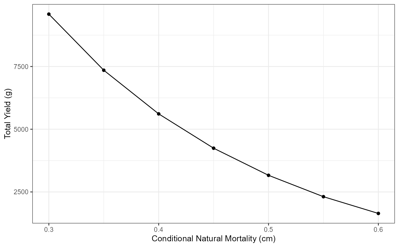
# Plot results
# Total Yield vs Conditional Natural Mortality (cm)
ggplot(data=Res_1,mapping=aes(x=cm,y=yieldTotal)) +
  geom_point() +
  geom_line() +
  labs(y="Total Yield (g)",x="Conditional Natural Mortality (cm)") +
  theme_bw()



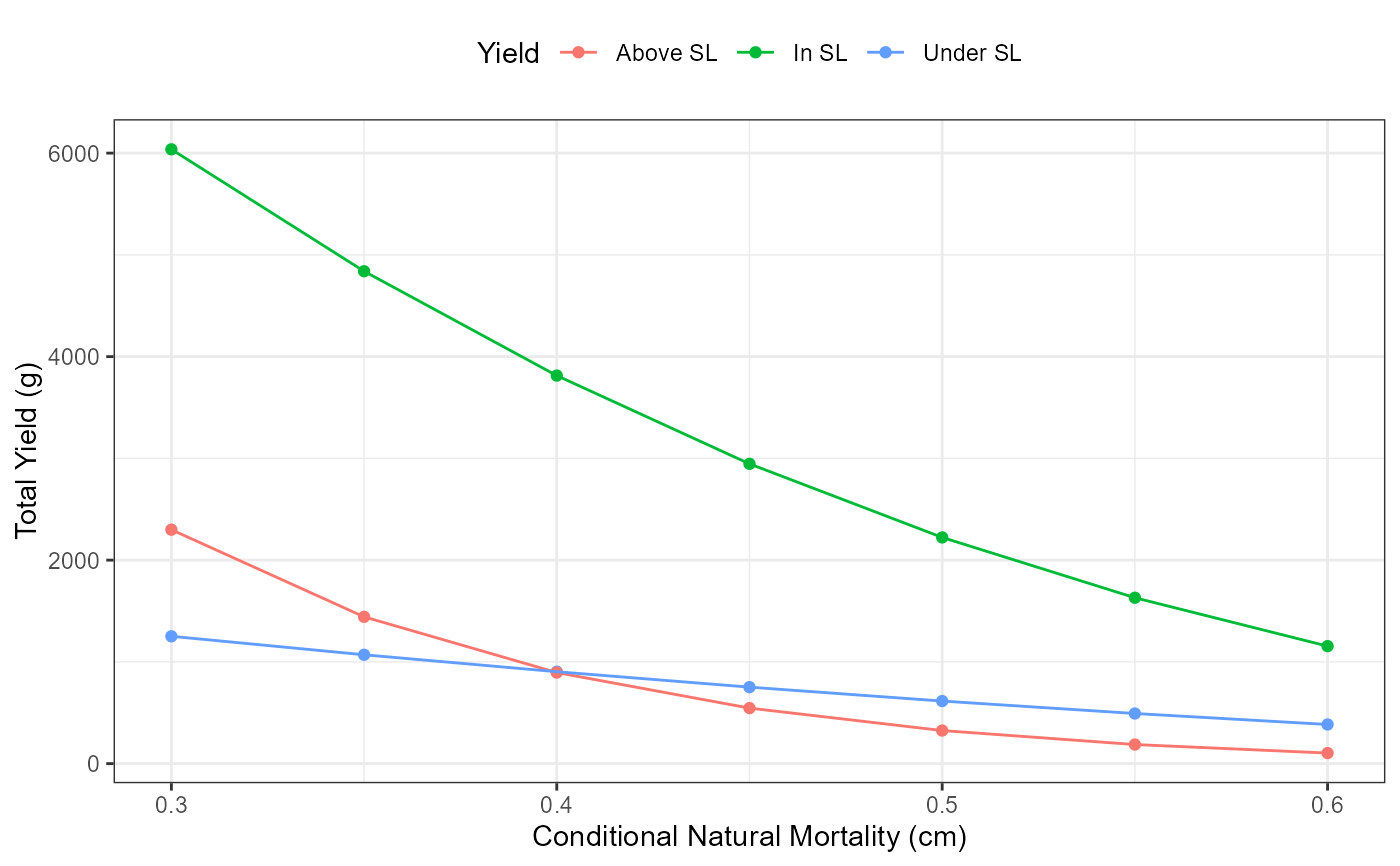
# Yield under, in, and above the slot limit vs Conditional Natural Mortality (cm)
# Select columns for plotting
plot_data <- Res_1 |>
  select(cm, yieldUnder, yieldIn, yieldAbove) |>
  pivot_longer(!cm, names_to="YieldCat",values_to="Yield")

# Generate plot
ggplot(data=plot_data,mapping=aes(x=cm,y=Yield,group=YieldCat,color=YieldCat)) +
  geom_point() +
  scale_color_discrete(name="Yield",labels=c("Above SL","In SL","Under SL"))+
  geom_line() +
  labs(y="Total Yield (g)",x="Conditional Natural Mortality (cm)") +
  theme_bw() +
  theme(legend.position = "top")+
  guides(color=guide_legend(title="Yield"))