Simulate expected yield under minimum length regulations using the Beverton-Holt Yield-per-Recruit model for a range of input parameters
Source:R/yprBH_MinLL.R
yprBH_MinLL.RdSimulate yield under minimum length regulations using the Beverton-Holt Yield-per-Recruit (YPR) model with (possibly) multiple values for minimum length limits for harvest (minLL), conditional fishing mortality (cf), and conditional natural mortality (cm).
Arguments
- minLL
A numeric vector of minimum length limits (in mm). All values must be less than
Linfinlhparms.- cf
A numeric vector of conditional fishing mortality. All values must be between 0 and 1 (inclusive).
- cm
A numeric vector of conditional natural mortality. All values must be between 0 and 1 (inclusive).
- lhparms
A named vector or list that contains values for each
N0,tmax,Linf,K,t0,LWalpha, andLWbeta. SeemakeLHfor definitions of these life history parameters. Also see details.- loi
A numeric vector of lengths (in mm) of interest. Used to determine number of fish that reach these lengths. All must be less than
Linfinlhparms.- matchRicker
A logical that indicates whether the yield function should match that in Ricker (1975). Defaults to
FALSE. See the FAMS vs Ricker article.
Value
A data.frame with the following calculated values:
yieldis the estimated yield (in g).exploitationis the exploitation rate.Nharvestis the number of harvested fish.Ndieis the number of fish that die of natural deaths.Ntis the number of fish at time tr (time they become harvestable size).avgwtis the average weight of fish harvested.avglenis the average length of fish harvested.tris the time for a fish to recruit to a minimum length limit (i.e., time to enter fishery).nAtxxxis the number that reach the length of interest supplied. There will be one column for each length of interest.Fis the instantaneous rate of fishing mortality.Mis the instantaneous rate of natural mortality.Zis the instantaneous rate of total mortality.Sis the (total) annual rate of survival.
For convenience the data.frame also contains the model input values (minLL, cf, andcm from input vectors; N0; Linf; K; t0; LWalpha; LWbeta; and tmax from lhparms).
The data.frame also contains a notes value which may contain abbreviations for "issues" that occurred when computing the results and were adjusted for. The possible abbreviates are as follows:
minLL>=Linf: The minimum length limit (minLL) being explored was greater than the given asymptotic mean length (Linf). For the purpose (only) of computing the time at recruitment to the fishery (tr) theLinfwas set tominLL+0.1.tr<t0: The age at recruitment to the fishery (tr) was less than the hypothetical time when the mean length is zero (t0). The fish can't recruit to the fishery prior to having length 0 sotrwas set tot0. This also assures that the time it takes to recruit to the fishery is greater than 0.Nt<0: The number of fish recruiting to the fishery was less than 0. There cannot be negative fish, soNtwas then set to 0.Nt>N0: The number of fish recruiting to the fishery was more than the number of fish recruited to the populations. Fish cannot be added to the cohort, soNtwas set toN0.Y=Infinite: The calculated yield (Y) was inifinity, which is impossible and suggests some other problem. Yield was set toNA.Y<0: The calculated yield (Y) was negative, which is impossible. Yield was set to 0.Nharv<0: The calculated number of fish harvested (Nharv) was negative, which is not possible. Number harvested was set to 0.Nharv>Nt: The calculated number of fish harvested (Nharv) was greater than the number of fish recruiting to the fishery, which is impossible. The number harvested was set to the number recruiting to the fishery.Ndie<0: The calculated number of fish recruiting to the fishery that died naturally (Ndie) was negative, which is not possible. Number that died was set to 0.Ndie>Nt: The calculated number of fish recruiting to the fishery that died naturally (Ndie) was greater than the number of fish recruiting to the fishery, which is impossible. The number that died was set to the number recruiting to the fishery.agvglen<minLL: The average length of harvested fish was less than the given minimum length limit being explored, which is not possible (with only legal harvest). The average length was set to the minimum length limit.
Details
Details will be filled out later.
Note that the main calculations are in the internal yprBH_func (use rFAMS:::yprBH_func to see that source code).
See also
yprBH_SlotLL for estimating yield with the yield-per-recruit model and a slot limit, or dpmBH_MinLL for estimating yield with a dynamic pool model using a minimum length limit.
See this demonstration page for more examples of this function.
Author
Jason C. Doll, jason.doll@fmarion.edu
Examples
# Load other required packages for organizing output and plotting
library(dplyr) ## for filter
library(ggplot2) ## for ggplot et al.
library(metR) ## geom_contour2
# Life history parameters to be used below
LH <- makeLH(N0=100,tmax=15,Linf=592,K=0.20,t0=-0.3,LWalpha=-5.528,LWbeta=3.273)
# Estimate yield for multiple values of minLL, cf, and cm
# # This is a minimal example, increments for minLL, cf, and cm would likely be smaller
# # to produce finer-scaled results.
minLL <- seq(from = 200, to = 550, by = 50)
cf <- seq(from = 0.1, to = 0.9, by = 0.1)
cm <- seq(from = 0.1, to = 0.9, by = 0.1)
loi <- c(400,450,500,550)
Res_1 <- yprBH_MinLL(minLL = minLL, cf = cf, cm = cm,
lhparms=LH, loi=loi)
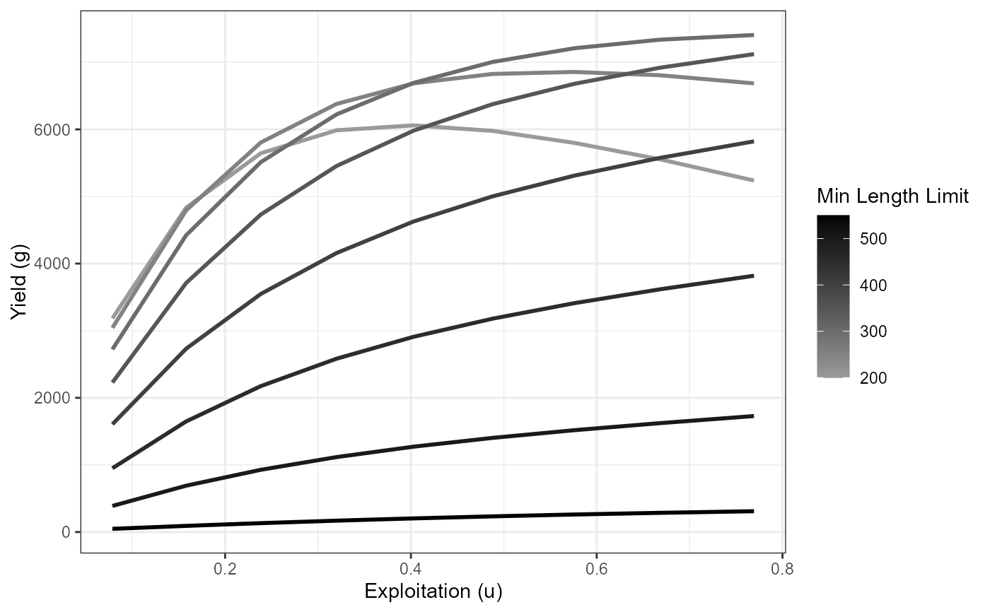
# Yield curves (yield vs exploitation) by varying minimum lengths,
# using cm=40
plot_dat <- Res_1 |> filter(cm==0.40)
ggplot(data=plot_dat,mapping=aes(y=yield,x=exploitation,
group=minLL,color=minLL)) +
geom_line(linewidth=1) +
scale_color_gradient2(high="black") +
xlab("Exploitation (u)")+
ylab("Yield (g)")+
labs(color="Min Length Limit") +
theme_bw()
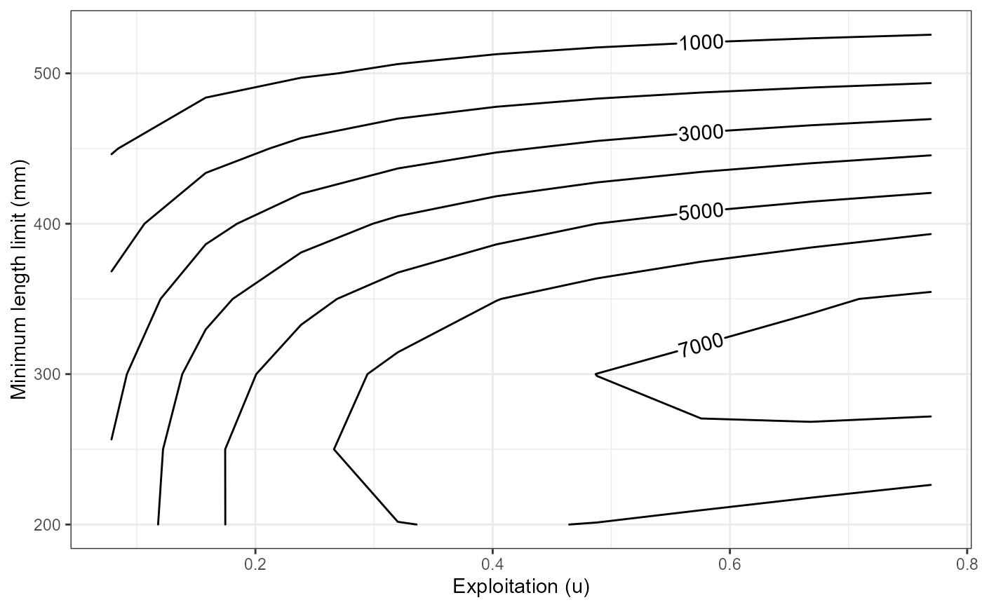
 # Yield isopleths for varying minLL and exploitation with cm=0.40
# # Using same data as previous example
ggplot(data=plot_dat,mapping=aes(x=exploitation,y=minLL,z=yield)) +
geom_contour2(aes(label = after_stat(level))) +
xlab("Exploitation (u)") +
ylab("Minimum length limit (mm)") +
theme_bw()
# Yield isopleths for varying minLL and exploitation with cm=0.40
# # Using same data as previous example
ggplot(data=plot_dat,mapping=aes(x=exploitation,y=minLL,z=yield)) +
geom_contour2(aes(label = after_stat(level))) +
xlab("Exploitation (u)") +
ylab("Minimum length limit (mm)") +
theme_bw()