Half-Life Property of K

Derek H. Ogle

Note

The following packages are loaded for use below. One function from FSA is also used below, but the full package was not loaded here. In addition, the plot was created with ggplot2, though the code is not shown in this post.

library(dplyr)  # for mutate()

Introduction

A colleague recently questioned whether \(\frac{log_{e}(2)}{K}\), where \(K\) is the Brody growth coefficient in the typical parameterization of the von Bertalanffy growth function, represents the “time it takes for a fish to grow from any length to a length halfway between the initial length and the asymptotic mean length (\(L_{\infty}\))”. This phenomenon is briefly illustrated below.

One Age

Create an R function for the typical von Bertalanffy growth function.

vb <- FSA::vbFuns()

Declare parameter values.

Linf <- 30
K <- 0.3
t0 <- -0.5

Predict mean length at some initial age.

initA <- 1
( initL <- vb(initA,Linf,K,t0) )

#R|  [1] 10.87116

Predict mean length at the initial age plus \(\frac{log_{e}(2)}{K}\).

nextA <- initA+log(2)/K
( nextL <- vb(nextA,Linf,K,t0) )

#R|  [1] 20.43558

Find the length that is halfway between the initial length and \(L_{\infty}\).¹

¹ all.equal() is used to test equality with a tolerance for machine precision.

( hwL <- mean(c(initL,Linf)) )

#R|  [1] 20.43558

all.equal(nextL,hwL)

#R|  [1] TRUE

Note that these last two values are equal, which illustrates the statement above about the “half-life” meaning of \(K\).

This can be repeated for a different initial age.

initA <- 7
( initL <- vb(initA,Linf,K,t0) )

#R|  [1] 26.83802

nextA <- initA+log(2)/K
( nextL <- vb(nextA,Linf,K,t0) )

#R|  [1] 28.41901

( hwL <- mean(c(initL,Linf)) )

#R|  [1] 28.41901

all.equal(nextL,hwL)

#R|  [1] TRUE

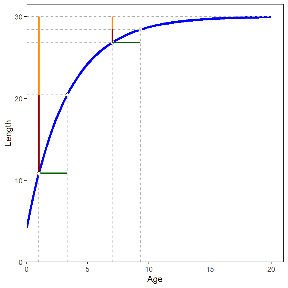
The two examples above can be examined in Figure 1, where the horizontal green lines illustrate the increase from the initial ages (e.g., 1 and 7) by \(\frac{log_{e}(2)}{K}\), the vertical red line is the change in length from the initial length to half of \(L_{\infty}\), and the vertical orange line is the remaining change in length to \(L_{\infty}\). The half-life property of \(K\) is thus illustrated by the equivalent lengths of the paired red and orange lines.

Figure 1: Demonstration of the half-life property of the K parameter in the von Bertalanffy growth function. (see text for description).

Multiple Ages

This process is repeated below for several initial age values. Note that the differences between the predicted mean length at the new age and the point halfway between the initial length and \(L_{\infty}\) are equal (within machine precision) for each initial age. Again, illustrating the statement about \(K\).

data.frame(initA=1:20) |>
  mutate(initL=vb(initA,Linf,K,t0),
         nextA=initA+log(2)/K,
         nextL=vb(nextA,Linf,K,t0),
         hwL=(initL+Linf)/2,
         areEqual=all.equal(nextL,hwL))

#R|     initA    initL     nextA    nextL      hwL areEqual
#R|  1      1 10.87116  3.310491 20.43558 20.43558     TRUE
#R|  2      2 15.82900  4.310491 22.91450 22.91450     TRUE
#R|  3      3 19.50187  5.310491 24.75093 24.75093     TRUE
#R|  4      4 22.22279  6.310491 26.11140 26.11140     TRUE
#R|  5      5 24.23850  7.310491 27.11925 27.11925     TRUE
#R|  6      6 25.73178  8.310491 27.86589 27.86589     TRUE
#R|  7      7 26.83802  9.310491 28.41901 28.41901     TRUE
#R|  8      8 27.65755 10.310491 28.82878 28.82878     TRUE
#R|  9      9 28.26467 11.310491 29.13234 29.13234     TRUE
#R|  10    10 28.71444 12.310491 29.35722 29.35722     TRUE
#R|  11    11 29.04763 13.310491 29.52382 29.52382     TRUE
#R|  12    12 29.29447 14.310491 29.64723 29.64723     TRUE
#R|  13    13 29.47733 15.310491 29.73866 29.73866     TRUE
#R|  14    14 29.61280 16.310491 29.80640 29.80640     TRUE
#R|  15    15 29.71315 17.310491 29.85658 29.85658     TRUE
#R|  16    16 29.78750 18.310491 29.89375 29.89375     TRUE
#R|  17    17 29.84257 19.310491 29.92129 29.92129     TRUE
#R|  18    18 29.88338 20.310491 29.94169 29.94169     TRUE
#R|  19    19 29.91360 21.310491 29.95680 29.95680     TRUE
#R|  20    20 29.93600 22.310491 29.96800 29.96800     TRUE

Different Parameters

The code below illustrates the same phenomenon for a very different set of parameter values.

Linf <- 300
K <- 0.9
t0 <- 1
data.frame(initA=1:20) |>
  mutate(initL=vb(initA,Linf,K,t0),
         nextA=initA+log(2)/K,
         nextL=vb(nextA,Linf,K,t0),
         hwL=(initL+Linf)/2,
         areEqual=all.equal(nextL,hwL))

#R|     initA    initL     nextA    nextL      hwL areEqual
#R|  1      1   0.0000  1.770164 150.0000 150.0000     TRUE
#R|  2      2 178.0291  2.770164 239.0146 239.0146     TRUE
#R|  3      3 250.4103  3.770164 275.2052 275.2052     TRUE
#R|  4      4 279.8383  4.770164 289.9192 289.9192     TRUE
#R|  5      5 291.8029  5.770164 295.9014 295.9014     TRUE
#R|  6      6 296.6673  6.770164 298.3337 298.3337     TRUE
#R|  7      7 298.6450  7.770164 299.3225 299.3225     TRUE
#R|  8      8 299.4491  8.770164 299.7246 299.7246     TRUE
#R|  9      9 299.7760  9.770164 299.8880 299.8880     TRUE
#R|  10    10 299.9089 10.770164 299.9545 299.9545     TRUE
#R|  11    11 299.9630 11.770164 299.9815 299.9815     TRUE
#R|  12    12 299.9849 12.770164 299.9925 299.9925     TRUE
#R|  13    13 299.9939 13.770164 299.9969 299.9969     TRUE
#R|  14    14 299.9975 14.770164 299.9988 299.9988     TRUE
#R|  15    15 299.9990 15.770164 299.9995 299.9995     TRUE
#R|  16    16 299.9996 16.770164 299.9998 299.9998     TRUE
#R|  17    17 299.9998 17.770164 299.9999 299.9999     TRUE
#R|  18    18 299.9999 18.770164 300.0000 300.0000     TRUE
#R|  19    19 300.0000 19.770164 300.0000 300.0000     TRUE
#R|  20    20 300.0000 20.770164 300.0000 300.0000     TRUE

Reuse

https://creativecommons.org/licenses/by/4.0/