Bayesian LVB I - brms

Jason Doll

Introduction

The use of Bayesian inference in fisheries biology has been increasing. For good reason, as there are many benefits to taking a Bayesian approach. I won’t go into those reasons here but you can read about them in Dorazio (2016) and Doll and Jacquemin (2018). This post assumes you have already decided to use Bayesian methods and will present how to estimate parameters of the von Bertalanffy growth model. Previous posts describe frequentist methods here and here

There are many programming languages that can be used to fit models with Bayesian inference. In this post, I will use Stan with the brms package. The brms packages is a wrapper for Stan that makes fitting simple models easier than writing the full model code. In a second post, I will show how the same model is fit using rstan and writing the full Stan model code. Although the brms package will write the full Stan model for you.

Both methods will fit the typical three parameter von Bertalanffy growth model

\[ TL_i=L_\infty * (1-e^{(-\kappa * (t_i-t_0))} ) \] where \(TL_i\) is total length of individual i, \(L_\infty\) is the average maximum length obtained, \(\kappa\) is the Brody growth coefficient, \(t_i\) is the age of individual i, and \(t_0\) is the theoretical age at zero length. To finish the model, an error term is added:

\[ TL_i=L_\infty * (1-e^{(-\kappa * (t_i-t_0))} + \epsilon_i) \] \[ \epsilon_i \sim normal(0,\sigma) \] Where \(\epsilon_i\) is a random error term for individual i with a mean of 0 and standard deviation \(\sigma\).

Prior probabilities

At the heart of Bayesian analysis is the prior probability distribution. This post will use non-informative prior probability distributions. When and how to use informative priors when fitting a von Bertalanffy growth model will be discussed in a future post. However, you can read about it in Doll and Jacquemin (2018). The prior probability distributions used in this post are:

Parameter	Prior Probability Distribution
\(L_\infty\)	normal(0,1000)
\(\kappa\)	normal(0,10)
\(t_0\)	normal(0,10)
\(\sigma\)	student-t(3,0,30)

Stan parameterizes the normal distribution with the mean and standard deviation and the student-t distribution with the degrees of freedom, mean, and standard deviation

Preliminaries

First step is to load the necessary packages

library(FSA)
library(FSAdata)   # for data
library(dplyr)     # for filter(), select()
library(ggplot2)   # for plotting
library(brms)      # for fitting Stan models
library(tidybayes) # for plotting posterior results
library(bayesplot) # for plotting posterior predictive checks

Data

The WalleyeErie2 data available in the FSAdata package was used in previous posts demonstrating von Bertalanffy growth models and will once again be used here. These data are Lake Erie Walleye (Sander vitreus) captured during October-November, 2003-2014. As before, the primary interest here is in the tl (total length in mm) and age variables. The data will also be filtered to focus only on female Walleye from location “1” captured in 2014.

data(WalleyeErie2,package="FSAdata")
wf14T <- WalleyeErie2 %>%
  filter(year==2014,sex=="female",loc==1) %>%
  select(-year,-sex,-setID,-loc,-grid)
headtail(wf14T)

#R|       tl    w      mat age
#R|  1   445  737 immature   2
#R|  2   528 1571   mature   4
#R|  3   380  506 immature   1
#R|  323 488 1089 immature   2
#R|  324 521 1408   mature   3
#R|  325 565 1745   mature   3

brms

The first step is to specify the formula using brmsformula(). The first argument below is the von Bertalanffy growth model, the second argument is to specify any hierarchical model of parameters (for example, estimate parameters by group or random effects), and the third is to tell brms that I want to fit a nonlinear model. Note in this example I do not specify any random effects for parameters. Also note that tl and age MUST be exactly how they are shown in the column headers of the data.

#Set formula
formula <- brmsformula(tl ~ Linf * (1 - exp(-K * (age - t0))),
                       Linf ~ 1, K ~ 1, t0 ~ 1, nl=TRUE)

The next step is to specify the prior probability distribution. Several parameters can’t be negative values so they are truncated using the lb=0 argument.

priors <- prior(normal(0,1000), nlpar="Linf", lb=0) +
          prior(normal(0,10), nlpar="K", lb=0) +
          prior(normal( 0,10), nlpar="t0") +
          prior(student_t(3,0,40), class=sigma)

An optional step is to specify initial values for the parameters. It is good practice to always specify initial values, particularly with non-linear and other complex models. I will fit the model using multiple chains and it is advisable to use different starting values for each chain. To accomplish this, we will specify a function and use a random number generator for each parameter. Adjust the range for the uniform distribution to cover a large range of values that make sense for your data. You can use other distributions as long as they match the declared range in the model code. In this example, I am using the random uniform function because \(L_\infty\) and \(\kappa\) are restricted to be positive in the model. Therefore, the starting value must be positive.

initsLst <- function() list(
  Linf=runif(1, 200, 800),
  K=runif(1, 0.05, 3.00),
  t0=rnorm(1, 0, 0.5)
)

Finally, use the brm() function to send the model, data, priors, initial values, and any specified settings to Stan and save the output in the fit1 object

fit1 <- brm(formula,            # calls the formula object created above
            family=gaussian(),  # specifies the error distribution
            data=wf14T,         # the data object
            prior=priors,       # the prior probability object 
            init=initsLst,      # the initial values object
            chains=3,           # number of chains, typically 3 to 4
            cores=3,            # number of cores for multi-core processing. Typically set to
                                # match number of chains. Adjust as needed to match the number
                                # of cores on your computer and number of chains
            iter=3000,          # number of iterations
            warmup=1000,        # number of warm up steps to discard
            control=list(adapt_delta=0.80,    # Adjustments to algorithm to 
                           max_treedepth=15)) # improve convergence.

Assess convergence

Before diving into the output, I like to examine the chains to see if they sufficiently mixed and reached a stationary posterior distribution.

plot(fit1)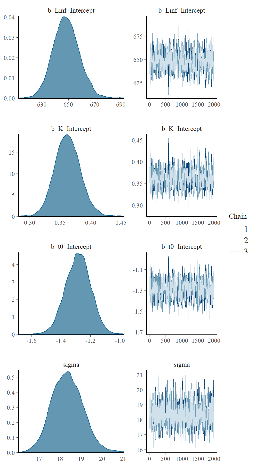

The chains appear to have mixed well for all parameters and reached a stationary posterior. This is seen by a unimodal distribution (on the left) and caterpillar plots for each parameter appear “on top” of each other (right).

We can also do a posterior predictive check to assess how well the model fit the data. A posterior predictive check compares observed data to predicted values based on the fitted model. If the model predicted values are “similar” to the observed data values then you can conclude the model fits the data well.

pp_check(fit1,ndraws=100)  # posterior predictive checks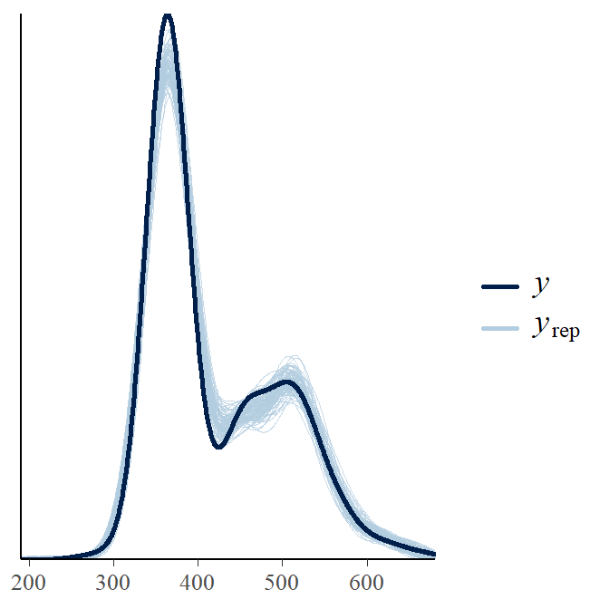

This figure shows two lines, one represents the data (y) and the other represents posterior predicted values from the model (y_rep). The y_rep generally follows the observed data so we can conclude the model fits the data well.

Posterior summary

Finally, we can examine the summary table of the output.

summary(fit1)

#R|   Family: gaussian 
#R|    Links: mu = identity; sigma = identity 
#R|  Formula: tl ~ Linf * (1 - exp(-K * (age - t0))) 
#R|           Linf ~ 1
#R|           K ~ 1
#R|           t0 ~ 1
#R|     Data: wf14T (Number of observations: 325) 
#R|    Draws: 3 chains, each with iter = 3000; warmup = 1000; thin = 1;
#R|           total post-warmup draws = 6000
#R|  
#R|  Population-Level Effects: 
#R|                 Estimate Est.Error l-95% CI u-95% CI Rhat Bulk_ESS Tail_ESS
#R|  Linf_Intercept   648.33      9.98   629.46   668.04 1.00     1364     2104
#R|  K_Intercept        0.36      0.02     0.32     0.40 1.00     1246     1743
#R|  t0_Intercept      -1.28      0.09    -1.45    -1.12 1.00     1349     1839
#R|  
#R|  Family Specific Parameters: 
#R|        Estimate Est.Error l-95% CI u-95% CI Rhat Bulk_ESS Tail_ESS
#R|  sigma    18.35      0.73    16.98    19.86 1.00     2048     2379
#R|  
#R|  Draws were sampled using sampling(NUTS). For each parameter, Bulk_ESS
#R|  and Tail_ESS are effective sample size measures, and Rhat is the potential
#R|  scale reduction factor on split chains (at convergence, Rhat = 1).

The summary table provides the point estimates, 95% credible intervals, Rhat values, and ESS. The Rhat values are another check to assess model convergence. It is generally accepted that you want Rhat values less than 1.10. Bulk_ESS and Tail_ESS are also used to assess convergence. Bulk_ESS and Tail_ESS refer to “Effective Sample Size.” Because of the nature of MCMC methods, each successive sample from the posterior will typically be autocorrelated within a chain. Autocorrelation within the chains can increase uncertainty in the estimates. One way to assessing how much autocorrelation is present and big of an effect it might be, is with the “Effective Sample Size.” ESS represents the number of independent draws from the posterior. The ESS will be lower than the actual number of draws and you are looking for a high ESS. It has been recommended that an ESS of 1,000 for each parameter is sufficient Bürkner (2017).

Posterior plotting

Now that we are convinced the model fit the data well, let’s plot the data and model predictions using the ggplot2 and tidybayes packages.

wf14T %>%
  add_predicted_draws(fit1) %>%  # adding the posterior distribution with tidybayes
  ggplot(aes(x=age, y=tl)) +  
  stat_lineribbon(aes(y=.prediction), .width=c(.95, .80, .50),  # regression line and CI
                  alpha=0.5, colour="black") +
  geom_point(data=wf14T, colour="darkblue", size=3) +   # raw data
  scale_fill_brewer(palette="Greys") +
  ylab("Total length (mm)\n") + 
  xlab("\nAge (years)") +
  theme_bw() +
  theme(legend.title=element_blank(),
        legend.position=c(0.15, 0.85))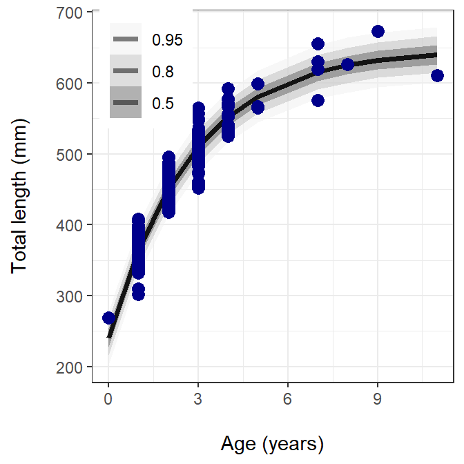

The figure above shows the observed data in blue circles, the prediction line as a solid black line, and the posterior prediction intervals (0.50, 0.80, and 0.95) in different shades of gray.

References

Bürkner, P.-C. 2017. Brms: An R Package for Bayesian Multilevel Models Using Stan. Journal of Statistical Software 80:1–28.

Doll, J. C., and S. J. Jacquemin. 2018. Introduction to Bayesian modeling and inference for fisheries scientists. Fisheries 43(3):152–161.

Dorazio, R. M. 2016. Bayesian data analysis in population ecology: Motivations, methods, and benefits. Population Ecology 58:31–44.

Reuse

https://creativecommons.org/licenses/by/4.0/

Citation

BibTeX citation:

@online{doll2024,
  author = {Doll, Jason},
  title = {Bayesian {LVB} {I} - Brms},
  date = {2024-02-05},
  url = {https://fishr-core-team.github.io/fishR//blog/posts/2024-2-5_LVB_brms},
  langid = {en}
}

For attribution, please cite this work as:

Doll, J. 2024, February 5. Bayesian LVB I - brms. https://fishr-core-team.github.io/fishR//blog/posts/2024-2-5_LVB_brms.