Vasquez et al. (2022) Kuskal-Wallis Results

Derek H. Ogle

Introduction

Vasquez et al. (2022) examined the nesting materials of Black-Crested Titmice (Baeolophus atricristatus) near San Marcos, Texas. In one part of their analysis they used a Kruskal-Wallis test to identify differences in total nest weight for nests from four different area types (based on a rural to urban gradient). They summarized their results in Panel A of their Figure 2. Here I recreate their statistics, but summarize the results differently.

The following packages are loaded for use below. A few functions from each of FSA, car, DescTools, and scales are used with :: such that the entire packages are not attached here.

library(tidyverse)  # for dplyr, ggplot2 packages

Data Wrangling

Vasquez et al. (2022) provided the raw data in their Data Supplement S1.

dat <- read.csv("JFWM-21-058.S1.csv")
names(dat)

#R|   [1] "Number"            "Location2"         "Location"         
#R|   [4] "Nest.Weight.and.P" "Plastic.Weight"    "Nest.Weight"      
#R|   [7] "Plastic"           "Cotton"            "Moss"             
#R|  [10] "Twigs"             "Leaves"            "Snake.Skin"       
#R|  [13] "Natural"           "Anthro"            "eggs.laid"        
#R|  [16] "eggs.hatch"        "Date"              "Julian"           
#R|  [19] "Beetle"            "First.Attempt"     "Second.Attempt"   
#R|  [22] "X2nd.Clutch"       "Photo"             "p.plastic"        
#R|  [25] "p.cotton"          "p.moss"            "p.twigs"          
#R|  [28] "p.leaves"          "p.snake"           "p.art"            
#R|  [31] "p.nat"             "total.prop"

There is both a Location and a Location2 variable in this data frame, but neither contains text that exactly match the “area types” shown in Vasquez et al. (2022).

xtabs(~Location+Location2,data=dat)

#R|              Location2
#R|  Location     Rural Semi Rural Semi Urban Urban
#R|    ACampus        0          0          0     7
#R|    BResidence     0          1         11     0
#R|    CPark          0          5          0     0
#R|    DFreeman      21          0          0     0

However, sample sizes for the Location variable groups match those in the paper. Therefore, I created Location3 by mapping the names in Location to the names used in the paper. I also turned Location3 into a factor to order the levels along the rural to urban gradient as Vasquez et al. (2022) did. Finally, for this post, I only focus on the total weight of the nest, so I only retained Nest.Weight and Location3 for further analysis.

dat2 <- dat |>
  mutate(Location3=plyr::mapvalues(Location,
                                   from=c("ACampus","BResidence","CPark","DFreeman"),
                                   to=c("Urban","Residential","Parks","Rural")),
         Location3=factor(Location3,levels=c("Rural","Parks","Residential","Urban"))) |>
  select(Location3,Nest.Weight)
FSA::headtail(dat2)

#R|       Location3 Nest.Weight
#R|  1        Urban        27.5
#R|  2        Urban        31.8
#R|  3        Urban        35.4
#R|  43 Residential        65.8
#R|  44 Residential        44.7
#R|  45 Residential        43.7

Kruskal-Wallis Test

Assumption Checking

Vasquez et al. (2022) chose to use a Kruskal-Wallis test¹ to determine if nest weights differed among area types because of concerns over normality and equal variances. They tested normality with a Shapiro-Wilk test, but this is difficult to do given the small sample sizes, especially in the “Parks” and “Urban” areas. Instead of the test I examined a density plot of total nest weight for each area type.

¹ I assume the reader is familiar with a Kruskal-Wallis Test. If not, this is one resource that may be useful.

ggplot(data=dat2,mapping=aes(x=Nest.Weight)) +
  geom_density(linewidth=0.75) +
  geom_rug(linewidth=0.75) +
  scale_x_continuous(name="Nest Weight (g)") +
  scale_y_continuous(expand=expansion(mult=c(0,0.05))) +
  facet_wrap(vars(Location3)) +
  theme_bw() +
  theme(axis.title.y=element_blank(),
        axis.text.y=element_blank())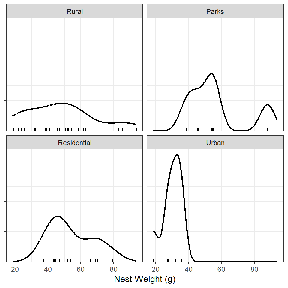

Alternatively, Q-Q plots² may be used to examine normality.

² I assume the reader is familiar with a Q_Q plot. If not, this is one resource that may be useful.

ggplot(data=dat2,mapping=aes(sample=Nest.Weight)) +
  geom_qq() +
  geom_qq_line(linewidth=0.75) +
  scale_x_continuous(name="Nest Weight (g)") +
  scale_y_continuous(expand=expansion(mult=c(0,0.05))) +
  facet_wrap(vars(Location3)) +
  theme_bw() +
  theme(axis.title.y=element_blank(),
        axis.text.y=element_blank())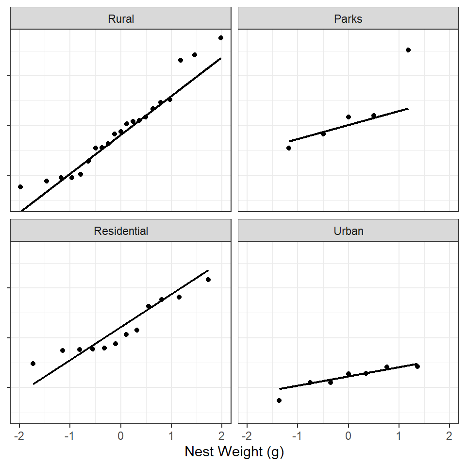

With either plot, the data do not appear to follow a normal distribution but, given the sample size, they do not look terribly non-normal either.

Vasquez et al. (2022) examined homogeneity of variances with the Bartlett test. I prefer to use Levene’s test for this purpose as it does not assume a normal distribution. Both bartlett.test() and leveneTest() (from car) require a formula of the form response~explanatory³ as the first argument and the corresponding data frame in data=.

³ Or dependent~independent.

bartlett.test(Nest.Weight~Location3,data=dat2)

#R|  
#R|     Bartlett test of homogeneity of variances
#R|  
#R|  data:  Nest.Weight by Location3
#R|  Bartlett's K-squared = 10.009, df = 3, p-value = 0.01849

car::leveneTest(Nest.Weight~Location3,data=dat2)

#R|  Levene's Test for Homogeneity of Variance (center = median)
#R|        Df F value Pr(>F)
#R|  group  3  2.2121 0.1012
#R|        41

Unfortunately, the two results give different answers, with Bartlett’s test suggesting unequal variances and Levene’s test suggesting the opposite.

Given these results it may have been appropriate to analyze these data with a one-way ANOVA. I suspect, however, that other variables in the data set more egregiously violated these assumptions and the authors wanted to use consistent methods for all variables. And, of course, using the Kruskal-Wallis test here a priori would not be incorrect, though there is some loss of power.

Kruskal-Wallis Test

The Kruskal-Wallis test may be performed with kruskal.test() using the same arguments as bartlett.test() or leveneTest() above.

kruskal.test(Nest.Weight~Location3,data=dat2)

#R|  
#R|     Kruskal-Wallis rank sum test
#R|  
#R|  data:  Nest.Weight by Location3
#R|  Kruskal-Wallis chi-squared = 11.571, df = 3, p-value = 0.009006

This result provides strong evidence that the median total nest weight is different for at least one of the area types.

Post-hoc Multiple Comparisons

Dunn’s test⁴ may be used, after a significant Kruskal-Wallis test, to determine which pairs of medians differ after adjusting for multiple comparisons. Dunn’s test is performed with dunnTest() from FSA using the same arguments as given to kruskal.test() above. As noted in the results below, dunnTest() defaults to using the “Holm” method to adjust for multiple comparisons. Other methods may be used with method=.⁵

⁴ I assume that the reader is familiar with Dunn’s Test. If not this is one resources that may be helpful.

⁵ See the possible methods with ?dunn.test::dunn.test.

FSA::dunnTest(Nest.Weight~Location3,data=dat2)

#R|             Comparison        Z     P.unadj      P.adj
#R|  1 Parks - Residential 0.233670 0.815241172 0.81524117
#R|  2       Parks - Rural 1.007831 0.313535451 0.62707090
#R|  3 Residential - Rural 1.042160 0.297337581 0.89201274
#R|  4       Parks - Urban 2.751550 0.005931397 0.02965699
#R|  5 Residential - Urban 3.126111 0.001771347 0.01062808
#R|  6       Rural - Urban 2.542487 0.011006664 0.04402666

From these results it is apparent that the median nest weight in the “Urban” areas differs from the other three area types, which all have statistically equal medians.

Displaying Results

Create Summary Data Frame

The Kruskal-Wallis test is a test of the equality of medians across groups. Thus, in my opinion, a summary graphic for this test should plot the medians with their respective confidence intervals. Computing the confidence intervals for medians across groups takes a bit of work in R. This process is described below.

The original data frame is converted to a list with separate vectors of nest weights for each area type.

tmp <- split(dat2$Nest.Weight,dat2$Location3)
tmp

#R|  $Rural
#R|   [1] 45.7 52.6 32.2 61.5 93.9 22.2 54.2 40.9 63.1 47.1 19.2 52.2 39.1 82.8 50.8
#R|  [16] 25.6 58.5 38.8 23.8 85.4 23.8
#R|  
#R|  $Parks
#R|  [1] 38.7 54.2 87.9 55.1 45.7
#R|  
#R|  $Residential
#R|   [1] 44.1 69.1 37.1 47.0 70.4 51.7 79.2 53.8 44.4 65.8 44.7 43.7
#R|  
#R|  $Urban
#R|  [1] 27.5 31.8 35.4 35.6 18.5 32.2 27.5

MedianCI() from DescTools may be used to compute the median and corresponding confidence interval for a vector of values. Below is an example for the “Urban” area. The default is to use a so-called “exact” method, but here I prefer to use “bootstrapping” instead so I include method="boot".

DescTools::MedianCI(tmp$Urban,method="boot")

#R|  median lwr.ci upr.ci 
#R|    31.8   28.2   36.1

sapply() can be used to “apply” MedianCI() to each item in the tmp list (so each area type) and return the result as a matrix.

tmp <- sapply(tmp,FUN=DescTools::MedianCI,method="boot")
tmp

#R|         Rural Parks Residential Urban
#R|  median  47.1  54.2       49.35  31.8
#R|  lwr.ci  40.0  20.5       31.25  28.2
#R|  upr.ci  55.4  69.7       54.45  36.1

However, the “median”, “lwr.ci”, and “upper.ci” should be the columns rather than the rows of this matrix. Thus, t() is used below to “transpose” the matrix which is then given to data.frame() to convert the matrix to a data frame.

sumNW <- t(tmp) |>
  data.frame()
sumNW

#R|              median lwr.ci upr.ci
#R|  Rural        47.10  40.00  55.40
#R|  Parks        54.20  20.50  69.70
#R|  Residential  49.35  31.25  54.45
#R|  Urban        31.80  28.20  36.10

Now, unfortunately, the area type names are row names and not a variable. Below, these row names are used to create a new Location3 variable and then converted to a factor with the levels controlled to match the authors’ order along a rural to urban gradient.

sumNW <- sumNW |>
  mutate(Location3=rownames(sumNW),
         Location3=factor(Location3,levels=c("Rural","Parks","Residential","Urban")))
sumNW

#R|              median lwr.ci upr.ci   Location3
#R|  Rural        47.10  40.00  55.40       Rural
#R|  Parks        54.20  20.50  69.70       Parks
#R|  Residential  49.35  31.25  54.45 Residential
#R|  Urban        31.80  28.20  36.10       Urban

Finally, a new variable is added that contains “significance letters” that communicate the results from Dunn’s Test above. Groups that have the same letter are statistically equal and those with different letters are statistically not equal. In this case, “Urban” was different than the other three which were all the same. Thus, “Urban” will have a unique letter that is different then the same letter used for the other three. I usually start the letters on the left, so “Rural” gets an “a” which it will share with “Parks” and “Residential” before “Urban” gets a “b.”

sumNW <- sumNW |>
  mutate(letsH=c("a","a","a","b"))
sumNW

#R|              median lwr.ci upr.ci   Location3 letsH
#R|  Rural        47.10  40.00  55.40       Rural     a
#R|  Parks        54.20  20.50  69.70       Parks     a
#R|  Residential  49.35  31.25  54.45 Residential     a
#R|  Urban        31.80  28.20  36.10       Urban     b

This data frame is the used to construct the summary graphic below.

Summary Graphic

I created the summary graphic below by …

Mapping Location3 to the x-axis for all geoms.
Mapping lwr.ci and upr.ci to ymin= and ymax=, respectively, in geom_errobar() to create the “intervals.” Here linewidth= was increased to make the interval lines “heavier”⁶ and width= was reduced to make the “caps” at the end of the interval lines narrower.
Mapping median to y= in geom_point() to place a point at the median. geom_point() came afer geom_errorbar() so that the point would be “on top” of the interval line. Here an open circle was used for the point with an inner portion a light gray and a black outline. The point was made larger than the default, as was the “stroke” used to draw the outline.⁷
Mapping letsH to labels= and upr.ci= to y in geom_text() to place the significance letters at the upper CI value. The vjust= was used to move the text up slightly⁸ and size= was used to show the letters in a 12 pt font.⁹
The y-axis was labeled, the breaks were controlled at 10 g intervals, the lower limit was constrained to be at 0, and the lower expansion was removed so that the x-axis was shown at a y of 0.
The x-axis was labeled.
The black-and-white theme was applied.
The axis titles were set a 14 pt font, and the axis tick mark labels were set to be black and in a 12 pt font.

⁶ The use of linewidth= was discussed in more detail in this post.

⁷ The use of size= and stroke= was discussed in more detail in this post.

⁸ The use of vjust= was discussed in more detail in this post.

⁹ The use of size= was discussed in more detail in this post.

ggplot(data=sumNW,mapping=aes(x=Location3)) +
  geom_errorbar(mapping=aes(ymin=lwr.ci,ymax=upr.ci),
                linewidth=0.75,width=0.1) +
  geom_point(mapping=aes(y=median),
             shape=21,size=2.5,stroke=1,
             fill="gray70",color="black") +
  geom_text(mapping=aes(label=letsH,y=upr.ci),vjust=-0.5,size=12/.pt) +
  scale_y_continuous(name="Median Nest Weight (g)",
                     breaks=scales::breaks_width(10),
                     limits=c(0,NA),expand=expansion(mult=c(0,0.05))) +
  scale_x_discrete(name="Area Type") +
  theme_bw() +
  theme(panel.grid=element_blank(),
        axis.title=element_text(size=14),
        axis.text=element_text(size=12,color="black"))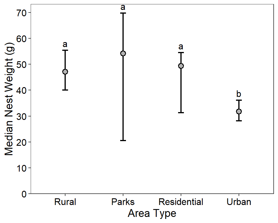

References

Vasquez, M. P., R. J. Rylander, J. M. Tleimat, and S. R. Fritts. 2022. Use of anthropogenic nest materials by Black-Crested Titmice along an urban gradient. Journal of Fish and Wildlife Management 13(1):236–242.

Reuse

https://creativecommons.org/licenses/by/4.0/

Citation

BibTeX citation:

@online{h. ogle2023,
  author = {H. Ogle, Derek},
  title = {Vasquez Et Al. (2022) {Kuskal-Wallis} {Results}},
  date = {2023-04-05},
  url = {https://fishr-core-team.github.io/fishR//blog/posts/2023-4-5_Vasquez2022_Fig2},
  langid = {en}
}

For attribution, please cite this work as:

H. Ogle, D. 2023, April 5. Vasquez et al. (2022) Kuskal-Wallis Results. https://fishr-core-team.github.io/fishR//blog/posts/2023-4-5_Vasquez2022_Fig2.