Nested X-Axis Labels

Derek H. Ogle

Introduction

Recently a Twitter follower asked …

Any thought on easy ways to add a second x axis? Ex: sampling periods (sequential) on x axis and reviewer asking for the correspoding year as an additional axis under/over primary axis. It appears…hard to do.

Here I explore a few different ways to do this.

The following packages are used here. Also note that a few functions from FSA and scales are used with :: so that the entire package is not attached here.

library(tidyverse)  # for ggplot2 and dplyr
library(ggh4x)      # for a variety of "hacks" described below

Option 1 - Facets

Example 1 - Bar Chart

Sample Data

Suppose you have very simple data where some numeric summary has been made for each group and that those groups are also categorized to a higher level. For example, total catch by species with species also categorized by family.¹

¹ Family is made a factor() here so that the order could be controlled (rather than alphabetical by default).

Code

dat1 <- data.frame(family=c("Centrarchid","Centrarchid","Percid","Percid","Esocid"),
                   species=c("Bluegill","Pumpkinseed","Walleye","Sauger","Muskellunge"),
                   catch=c(34,45,23,36,7)) |>
  mutate(family=factor(family,levels=c("Centrarchid","Percid","Esocid")))
dat1

#R|         family     species catch
#R|  1 Centrarchid    Bluegill    34
#R|  2 Centrarchid Pumpkinseed    45
#R|  3      Percid     Walleye    23
#R|  4      Percid      Sauger    36
#R|  5      Esocid Muskellunge     7

A simple bar chart of these data is created with geom_col() with species mapped to the x-axis and catch mapped to the y-axis. Here I provided a title for the y-axis, removed the lower expansion and reduce the upper expansion of the y-axis, applied the classic theme, increased the size of the axis title and tick mark text, made the axis titles bold, made the tick mark text black, and removed the x-axis title.

ggplot(data=dat1,mapping=aes(x=species,y=catch)) +
  geom_col() +
  scale_y_continuous(name="Total catch",expand=expansion(mult=c(0,0.025))) +
  theme_classic() +
  theme(axis.title=element_text(size=12,face="bold"),
        axis.title.x=element_blank(),
        axis.text=element_text(size=10,color="black"))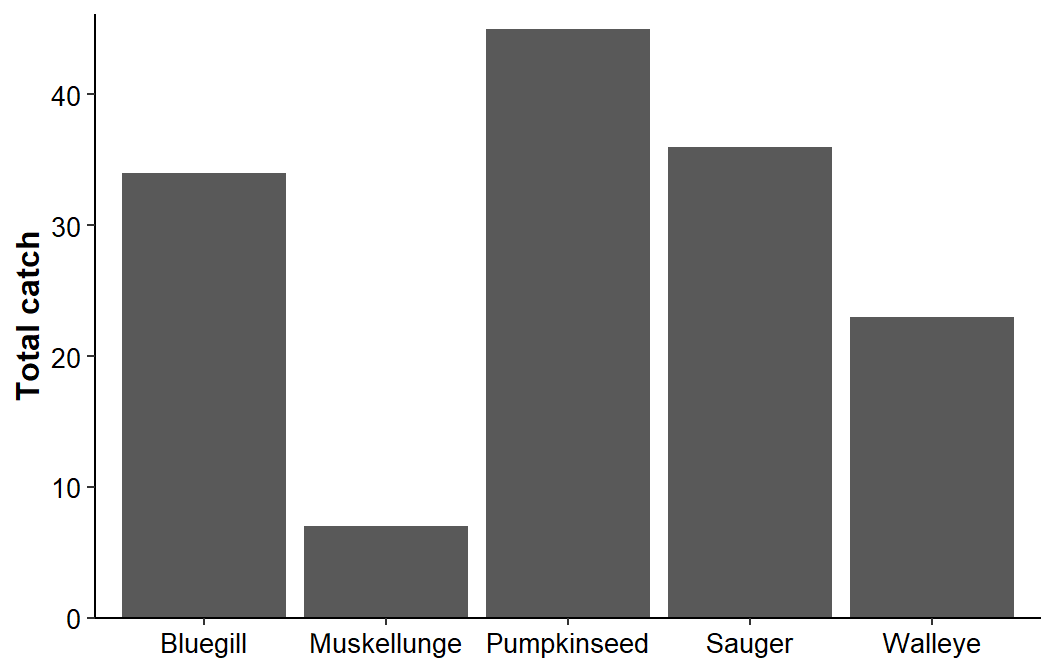

What the Twitter follower would want in this case is another layer of x-axis labels that would succinctly identify the family for each species.

Specifying Facets

Faceting provides one option for applying these labels. Below I added one row of facets based on the family name with facet_grid().

ggplot(data=dat1,mapping=aes(x=species,y=catch)) +
  geom_col() +
  scale_y_continuous(name="Total catch",expand=expansion(mult=c(0,0.025))) +
  facet_grid(cols=vars(family)) +
  theme_classic() +
  theme(axis.title=element_text(size=12,face="bold"),
        axis.title.x=element_blank(),
        axis.text=element_text(size=10,color="black"))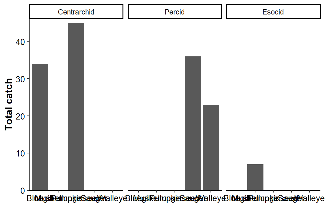

This does not look immediately helpful!! However, adding scales="free_x" to facet_grid() reduces each x-axis to only the species present in that facet (i.e., family).

ggplot(data=dat1,mapping=aes(x=species,y=catch)) +
  geom_col() +
  scale_y_continuous(name="Total catch",expand=expansion(mult=c(0,0.025))) +
  facet_grid(cols=vars(family),scales="free_x") +
  theme_classic() +
  theme(axis.title=element_text(size=12,face="bold"),
        axis.title.x=element_blank(),
        axis.text=element_text(size=10,color="black"))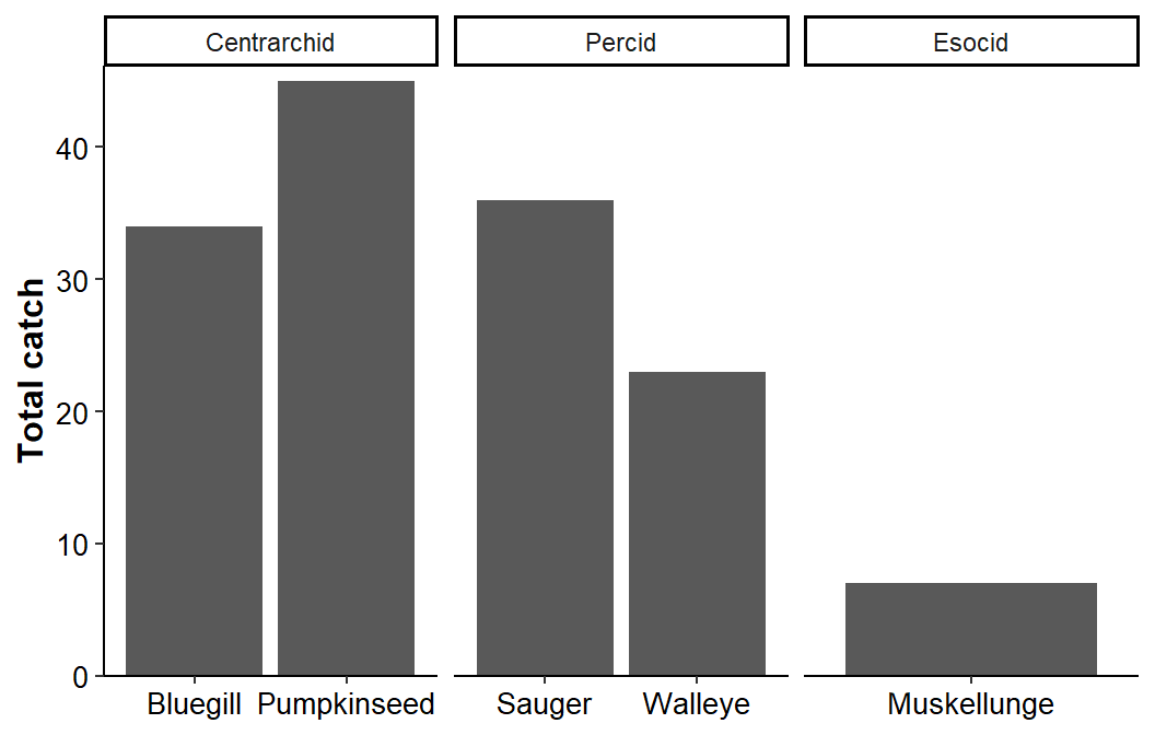

Adding space=free_x to facet_grid() ensures that the “bars” in each facet are the same width by adjusting the facet width to match the space needed to show just the data for that facet.

ggplot(data=dat1,mapping=aes(x=species,y=catch)) +
  geom_col() +
  scale_y_continuous(name="Total catch",expand=expansion(mult=c(0,0.025))) +
  facet_grid(cols=vars(family),scales="free_x",space="free_x") +
  theme_classic() +
  theme(axis.title=element_text(size=12,face="bold"),
        axis.title.x=element_blank(),
        axis.text=element_text(size=10,color="black"))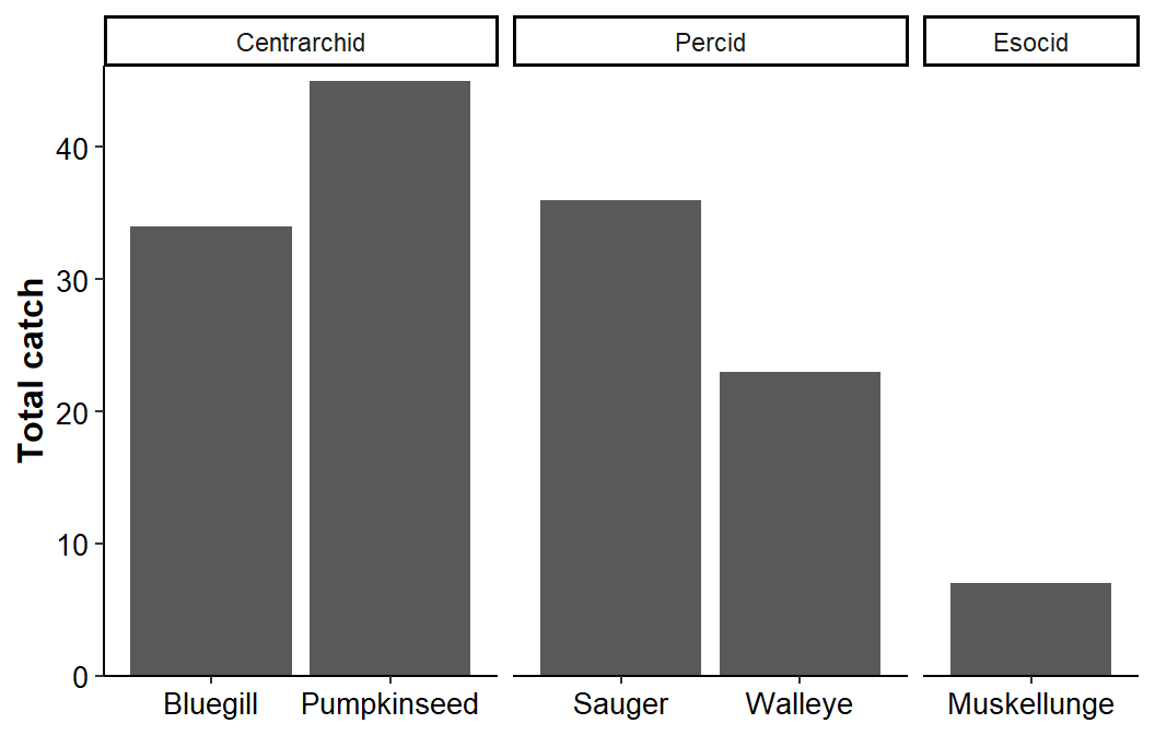

Finally, adding switch="x" to facet_grid() moves the facet strip labels to the bottom of the plot area for each facet.

ggplot(data=dat1,mapping=aes(x=species,y=catch)) +
  geom_col() +
  scale_y_continuous(name="Total catch",expand=expansion(mult=c(0,0.025))) +
  facet_grid(cols=vars(family),scales="free_x",space="free_x",switch="x") +
  theme_classic() +
  theme(axis.title=element_text(size=12,face="bold"),
        axis.title.x=element_blank(),
        axis.text=element_text(size=10,color="black"))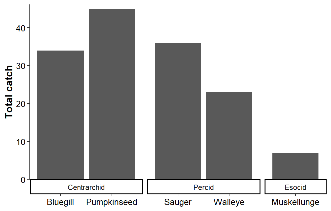

The next step is to move the facet strip labels “outside”² the axis tick mark labels with strip.placement='outside' in theme(). The facet strip “box” was also removed with strip.background.x= and the facet strip text was altered with strip.text=.

² Rather than the default “inside”.

ggplot(data=dat1,mapping=aes(x=species,y=catch)) +
  geom_col() +
  scale_y_continuous(name="Total catch",expand=expansion(mult=c(0,0.025))) +
  facet_grid(cols=vars(family),scales="free_x",space="free_x",switch="x") +
  theme_classic() +
  theme(axis.title=element_text(size=12,face="bold"),
        axis.title.x=element_blank(),
        axis.text=element_text(size=10,color="black"),
        strip.placement='outside',
        strip.background.x=element_blank(),
        strip.text=element_text(size=12,color="black",face="bold"))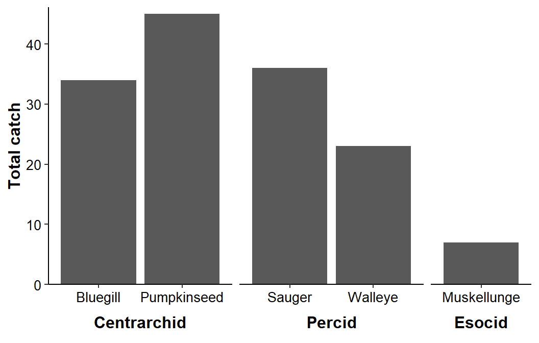

Finally, facets were “smushed” together so that the x-axis looks continuous by reducing panel.spacing.x= to 0.

ggplot(data=dat1,mapping=aes(x=species,y=catch)) +
  geom_col() +
  scale_y_continuous(name="Total catch",expand=expansion(mult=c(0,0.025))) +
  facet_grid(cols=vars(family),scales="free_x",space="free_x",switch="x") +
  theme_classic() +
  theme(axis.title=element_text(size=12,face="bold"),
        axis.title.x=element_blank(),
        axis.text=element_text(size=10,color="black"),
        strip.placement='outside',
        strip.background.x=element_blank(),
        strip.text=element_text(size=12,color="black",face="bold"),
        panel.spacing.x=unit(0,"pt"))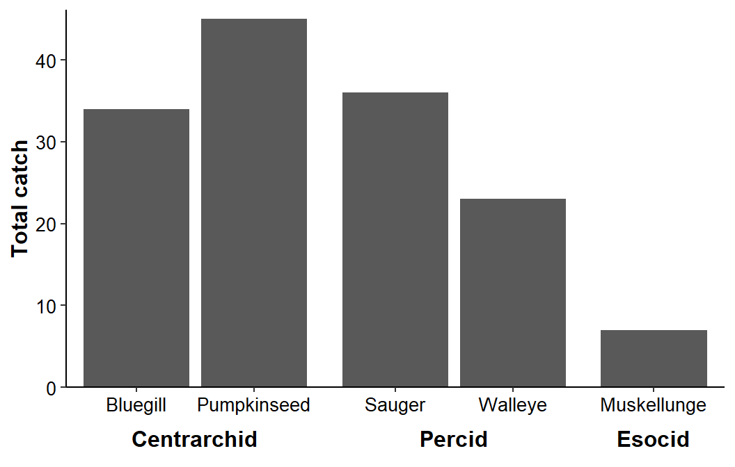

The family categorization could be further highlighted with a fill= color mapped to family.

ggplot(data=dat1,mapping=aes(x=species,y=catch,fill=family)) +
  geom_col(color="black") +
  scale_y_continuous(name="Total catch",expand=expansion(mult=c(0,0.025))) +
  scale_fill_grey(start=0.1,end=0.5) +
  facet_grid(cols=vars(family),scales="free_x",space="free_x",switch="x") +
  theme_classic() +
  theme(axis.title=element_text(size=12,face="bold"),
        axis.title.x=element_blank(),
        axis.text=element_text(size=10,color="black"),
        strip.placement='outside',
        strip.background.x=element_blank(),
        strip.text=element_text(size=12,color="black",face="bold"),
        panel.spacing.x=unit(0,"pt"),
        legend.position="none")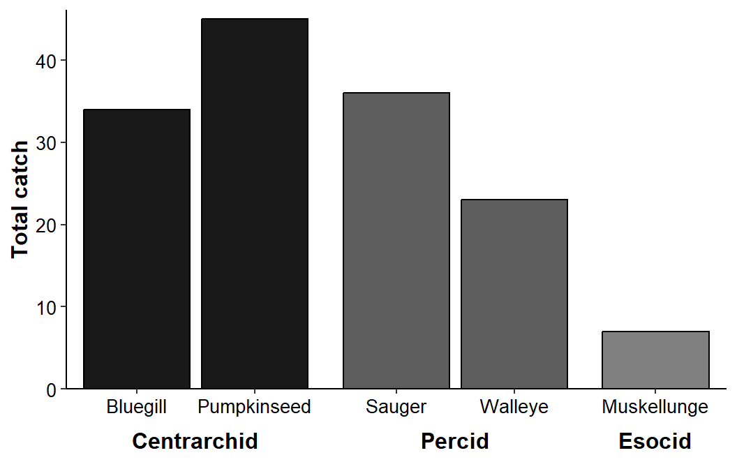

Open Question

I could not, using this method, figure out how to reduce the inter-facet gap between bars so that it matched the intra-facet gap between bars.

Example 2 - Bar Chart with Dates

The Twitter follower’s questions was about dates. So, imagine data that is the total catch of a species from the second(ish) week of each month over a few year period.

Code

dat2 <- data.frame(sample_date=seq(as.Date("2020-8-12"),
                                   as.Date("2022-4-7"),by="month")) |>
  mutate(sample_date=sample_date-sample((-5:5),length(sample_date),replace=TRUE),
         catch=round(runif(length(sample_date),50,150)))

FSA::headtail(dat2)

#R|     sample_date catch
#R|  1   2020-08-14    73
#R|  2   2020-09-15   110
#R|  3   2020-10-15   149
#R|  18  2022-01-14   131
#R|  19  2022-02-07    83
#R|  20  2022-03-10    54

Now extract the month and year from the sample dates.

dat2 <- dat2 |>
  mutate(mon=month(sample_date,label=TRUE),
         yr=year(sample_date))
FSA::headtail(dat2)

#R|     sample_date catch mon   yr
#R|  1   2020-08-14    73 Aug 2020
#R|  2   2020-09-15   110 Sep 2020
#R|  3   2020-10-15   149 Oct 2020
#R|  18  2022-01-14   131 Jan 2022
#R|  19  2022-02-07    83 Feb 2022
#R|  20  2022-03-10    54 Mar 2022

A plot using the faceting method is created below.

ggplot(data=dat2,mapping=aes(x=mon,y=catch,fill=factor(yr))) +
  geom_col() +
  scale_y_continuous(name="Total catch",expand=expansion(mult=c(0,0.25))) +
  scale_fill_viridis_d(begin=0.1,end=0.5) +
  facet_grid(cols=vars(yr),space='free_x',scales='free_x',switch='x') +
  theme_classic() +
  theme(axis.title=element_text(size=12,face="bold"),
        axis.title.x=element_blank(),
        axis.text=element_text(size=10,color="black"),
        strip.placement='outside',
        strip.background.x=element_blank(),
        strip.text=element_text(size=12,color="black",face="bold"),
        panel.spacing.x=unit(0,"pt"),
        legend.position="none")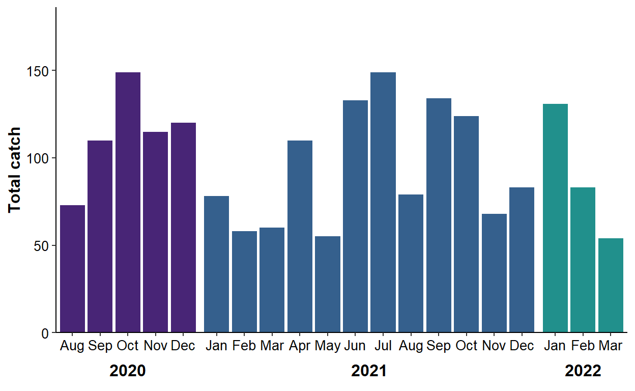

Option 2 - ggh4x

Example 1 - Bar Chart

The ggh4x package provides guide_axis_nested() and related helpers for creating the secondary x-axis. This function, however, is predicated on plotting the interaction between the variables that defined the primary and secondary labels on the x-axis. An “interaction” is created with interaction() with, for these purposes, the nested variable listed second. For further below it is important to note that the parts of the interactions are separated by a single dot/period.

dat1 <- dat1 |>
  mutate(sfint=interaction(species,family))
dat1

#R|         family     species catch                   sfint
#R|  1 Centrarchid    Bluegill    34    Bluegill.Centrarchid
#R|  2 Centrarchid Pumpkinseed    45 Pumpkinseed.Centrarchid
#R|  3      Percid     Walleye    23          Walleye.Percid
#R|  4      Percid      Sauger    36           Sauger.Percid
#R|  5      Esocid Muskellunge     7      Muskellunge.Esocid

The basic bar chart from above is modified by mapping this interaction variable, rather than species, to the x-axis.

ggplot(data=dat1,mapping=aes(x=sfint,y=catch)) +
  geom_col() +
  scale_y_continuous(name="Total catch",expand=expansion(mult=c(0,0.025))) +
  theme_classic() +
  theme(axis.title=element_text(size=12,face="bold"),
        axis.title.x=element_blank(),
        axis.text=element_text(size=10,color="black"))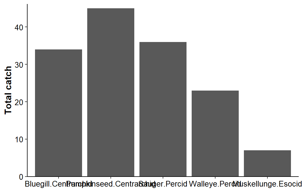

The parts of the interactions can be disentangled and turned into nested axes by setting guide_axis_nested() equal to guide= in scale_x_discrete(). Note that delim="." is used in guide_axis_nested() because the parts of the interaction were separated with a single dot/period.

ggplot(data=dat1,mapping=aes(x=sfint,y=catch)) +
  geom_col() +
  scale_y_continuous(name="Total catch",expand=expansion(mult=c(0,0.025))) +
  scale_x_discrete(guide=guide_axis_nested(delim=".")) +
  theme_classic() +
  theme(axis.title=element_text(size=12,face="bold"),
        axis.title.x=element_blank(),
        axis.text=element_text(size=10,color="black"))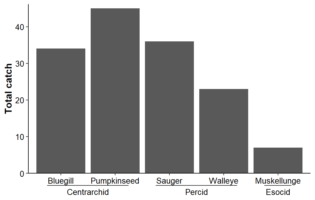

The primary tick mark labels are controlled with axis.text.x= which inherits from axis.text= if not given. Thus, the “species” labels are 10 pt black as defined above. The secondary tick mark labels inherit from axis.text.x= unless modifications are made in ggh4x.axis.nesttext.x= using element_text(). Below the “family” labels are set to 12 pt bold text.³ Finally, the line that separates the levels of labels is controlled with element_line() in ggh4x.axis.nestline.x=. The line is made slightly heavier below for illustration.

³ And will be black because axis.text= was set to black.

ggplot(data=dat1,mapping=aes(x=sfint,y=catch)) +
  geom_col() +
  scale_y_continuous(name="Total catch",expand=expansion(mult=c(0,0.025))) +
  scale_x_discrete(guide=guide_axis_nested(delim=".")) +
  theme_classic() +
  theme(axis.title=element_text(size=12,face="bold"),
        axis.title.x=element_blank(),
        axis.text=element_text(size=10,color="black"),
        ggh4x.axis.nesttext.x=element_text(size=12,face="bold"),
        ggh4x.axis.nestline.x=element_line(linewidth=0.75))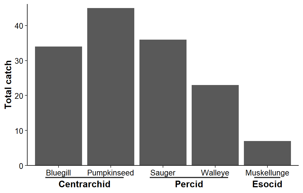

Open Question

I could not, using this method, figure out how to make the line between the two levels of labels longer. For example, I would prefer the “Centrarchid” line to extend further right to more completely cover “Pumpkinseed.”

Example 2 – Bar Chart with Dates

The data frame used for Option 1 must be modified to include the interaction between the mon and yr for use with ggh4x.

dat2 <- dat2 |>
  mutate(myint=interaction(mon,yr))
FSA::headtail(dat2)

#R|     sample_date catch mon   yr    myint
#R|  1   2020-08-14    73 Aug 2020 Aug.2020
#R|  2   2020-09-15   110 Sep 2020 Sep.2020
#R|  3   2020-10-15   149 Oct 2020 Oct.2020
#R|  18  2022-01-14   131 Jan 2022 Jan.2022
#R|  19  2022-02-07    83 Feb 2022 Feb.2022
#R|  20  2022-03-10    54 Mar 2022 Mar.2022

A plot using ggh4x is created below.

ggplot(data=dat2,mapping=aes(x=myint,y=catch,fill=factor(yr))) +
  geom_col() +
  scale_y_continuous(name="Total catch",expand=expansion(mult=c(0,0.25))) +
  scale_fill_viridis_d(begin=0.1,end=0.5) +
  scale_x_discrete(guide=guide_axis_nested(delim=".")) +
  theme_classic() +
  theme(axis.title=element_text(size=12,face="bold"),
        axis.title.x=element_blank(),
        axis.text=element_text(size=10,color="black"),
        ggh4x.axis.nesttext.x=element_text(size=12,face="bold"),
        ggh4x.axis.nestline.x=element_line(linewidth=0.75),
        legend.position="none")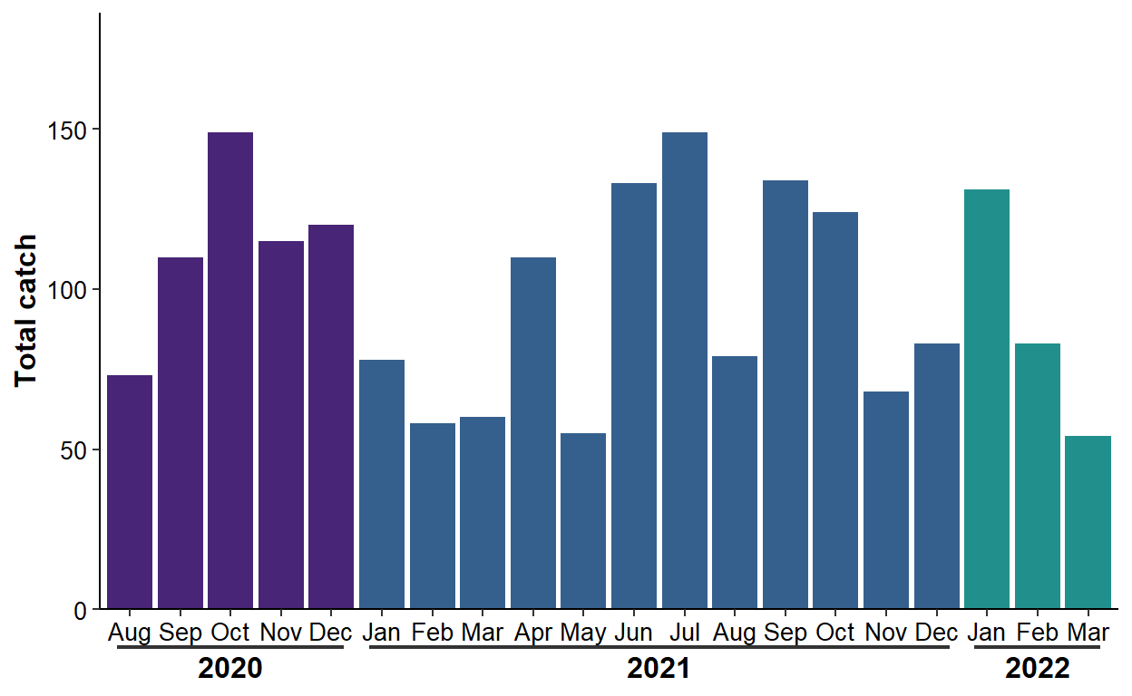

Option 3 - Manual Placement

Example 1 - Bar Chart

A third options is to create space below the x-axis and “place” the secondary axis “manually.” Before creating this space it is important to order primary axis labels so that categories to be grouped by the secondary level are next to each other. In this example, the species variable must be converted to a factor with the levels controlled so that families are grouped together.

dat1 <- dat1 |>
  mutate(species=factor(species,levels=c("Bluegill","Pumpkinseed",
                                         "Walleye","Sauger",
                                         "Muskellunge")))

Space below the x-axis is created by increasing the bottom margin around the plot with plot.margin= in theme(). Below the bottom margin was increased to two “lines” and the other margins were set to one “line”.⁴

⁴ The top, left, and right margins are defined by t=, l= and r= in margin().

ggplot(data=dat1,mapping=aes(x=species,y=catch)) +
  geom_col() +
  scale_y_continuous(name="Total catch",expand=expansion(mult=c(0,0.025))) +
  theme_classic() +
  theme(axis.title=element_text(size=12,face="bold"),
        axis.title.x=element_blank(),
        axis.text=element_text(size=10,color="black"),
        plot.margin=margin(b=2,t=1,l=1,r=1,unit="lines"))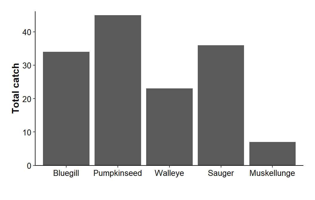

Plot “clipping” must be turned off with clip="off" in coord_caresian() to be able to place “objects” in the space just created.⁵ In addition, the y-axis limits should be set with ylim= in coord_cartesian() so that the y-axis limits do not change as labels are added beneath the x-axis. As a demonstration, I placed my name at the x=1.5 and y=-5 coordinate.

⁵ Because that space is outside of the main plot area.

ggplot(data=dat1,mapping=aes(x=species,y=catch)) +
  geom_col() +
  scale_y_continuous(name="Total catch",expand=expansion(mult=c(0,0.025))) +
  theme_classic() +
  theme(axis.title=element_text(size=12,face="bold"),
        axis.title.x=element_blank(),
        axis.text=element_text(size=10,color="black"),
        plot.margin=margin(b=2,t=1,l=1,r=1,unit="lines")) +
  coord_cartesian(ylim=c(0,NA),clip="off") +
  annotate(geom="text",x=1.5,y=-5,label="Derek",color="red",fontface="bold")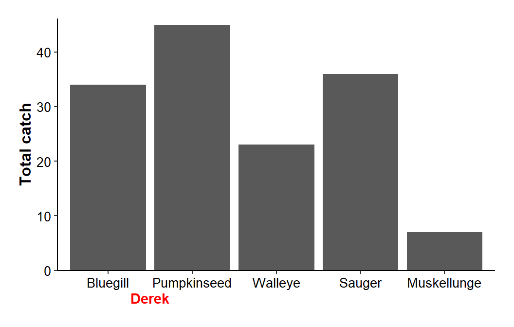

Choosing a value for the y-coordinate beneath the axis is largely a matter of trial-and-error after an initial first guess. The x-coordinate, though, can largely be determined from the x-axis. The levels for a factor such as species are recorded as integers “behind-the-scenes.” In this example, a “Bluegill” is defined with a “1” as it is the first level and its bar will be above an invisible “1” on the x-axis. Thus, placing my name at x=1.5 centers it between the first and second bars.

Here I want to create a secondary axis similar to what ggh4x produced – a line segment with a label underneath it. The first segment for the secondary axis should cover “Bluegill” and “Pumpkinseed.” Thus, it should start a little below 1 and end a little above 2. Other segments are defined similarly and stored in a data frame below.

x2lns <- data.frame(xstart=c(0.55,2.55,4.55),
                    xend=c(2.45,4.45,5.45))
x2lns

#R|    xstart xend
#R|  1   0.55 2.45
#R|  2   2.55 4.45
#R|  3   4.55 5.45

At first, I roughly guess at starting and ending points and then come back to adjust these values if the lines need to be extended or shortened to look good. These segments are added to the plot with geom_segment() using this new data frame with the variables mapped appropriately. I set y= and yend= outside of aes() as the y-coordinate is constant for all these segments. Finally, the segment was made slightly heavier.

ggplot(data=dat1,mapping=aes(x=species,y=catch)) +
  geom_col() +
  scale_y_continuous(name="Total catch",expand=expansion(mult=c(0,0.025))) +
  theme_classic() +
  theme(axis.title=element_text(size=12,face="bold"),
        axis.title.x=element_blank(),
        axis.text=element_text(size=10,color="black"),
        plot.margin=margin(b=2,t=1,l=1,r=1,unit="lines")) +
  coord_cartesian(ylim=c(0,NA),clip="off") +
  geom_segment(data=x2lns,mapping=aes(x=xstart,xend=xend),y=-5,yend=-5,
               linewidth=0.75)

Once the segments are set as desired, another data frame is created that has the x-axis coordinate and text for the secondary axis label. Below, the coordinate was found by averaging xstart and xend for each segment in x2lns.⁶ The text for the labels was then entered manually.

⁶ This x coordinates in this data frame could have been entered manually, but computing the average makes it easier to put the label in the center of the segment.

x2lbls <- x2lns |>
  rowwise() |>
  summarize(x=mean(c(xstart,xend))) |>
  ungroup() |>
  mutate(lbl=c("Centrarchid","Percid","Esocid"))
x2lbls

#R|  # A tibble: 3 × 2
#R|        x lbl        
#R|    <dbl> <chr>      
#R|  1   1.5 Centrarchid
#R|  2   3.5 Percid     
#R|  3   5   Esocid

These labels are then added with geom_text() using the new data frame with the variables mapped appropriately. Again, y= was set outside of aes() as this coordinate is constant for all labels. The text was adjusted to be a 12 pt bold.

ggplot(data=dat1,mapping=aes(x=species,y=catch)) +
  geom_col() +
  scale_y_continuous(name="Total catch",expand=expansion(mult=c(0,0.025))) +
  theme_classic() +
  theme(axis.title=element_text(size=12,face="bold"),
        axis.title.x=element_blank(),
        axis.text=element_text(size=10,color="black"),
        plot.margin=margin(b=2,t=1,l=1,r=1,unit="lines")) +
  coord_cartesian(ylim=c(0,NA),clip="off") +
  geom_segment(data=x2lns,mapping=aes(x=xstart,xend=xend),y=-5,yend=-5,
               linewidth=0.75) +
  geom_text(data=x2lbls,mapping=aes(x=x,label=lbl),y=-8,
            size=12/.pt,fontface="bold")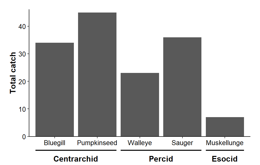

Important

Choosing how much to increase the bottom margin and choosing the x- and y-coordinates for the secondary x-axis labels with this method is largely a matter of trial-and-error.

Example 3 - Line Plot

Options 1 and 2 cannot handle situations where the plot is not “discrete.”⁷ For example, suppose that a line plot of total catch in dat2 by sample date (rather than month) is desired.

⁷ At least, I could not make them work for these situations.

ggplot(data=dat2,mapping=aes(x=sample_date,y=catch)) +
  geom_line(linewidth=1) +
  scale_x_date(breaks=scales::breaks_width("month"),
               labels=scales::label_date("%b %y"),expand=expansion(mult=0.01)) +
  scale_y_continuous(name="Total catch",limits=c(0,200),expand=expansion(mult=0)) +
  theme_classic() +
  theme(axis.title=element_text(size=12,face="bold"),
        axis.title.x=element_blank(),
        axis.text=element_text(size=10,color="black"))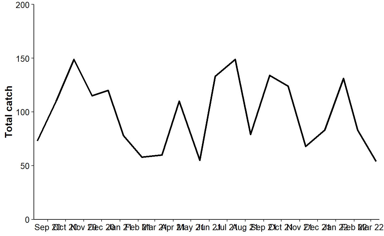

However, the x-axis is cluttered and suppose that a reviewer wants the months shown on the x-axis ticks with years as a secondary axis below that. The methods from above may be tried, but faceting clearly does not work (see below) and I could not get the ggh4x method to work with scale_x_date().

ggplot(data=dat2,mapping=aes(x=sample_date,y=catch)) +
  geom_line(linewidth=1) +
  scale_x_date(breaks=scales::breaks_width("month"),
               labels=scales::label_date("%b"),expand=expansion(mult=0.01)) +
  scale_y_continuous(name="Total catch",limits=c(0,200),expand=expansion(mult=0)) +
  facet_grid(cols=vars(yr),space='free_x',scales='free_x',switch='x') +
  theme_classic() +
  theme(axis.title=element_text(size=12,face="bold"),
        axis.title.x=element_blank(),
        axis.text=element_text(size=10,color="black"),
        strip.placement='outside',
        strip.background.x=element_blank(),
        strip.text=element_text(size=12,color="black",face="bold"),
        panel.spacing.x=unit(0,"pt"))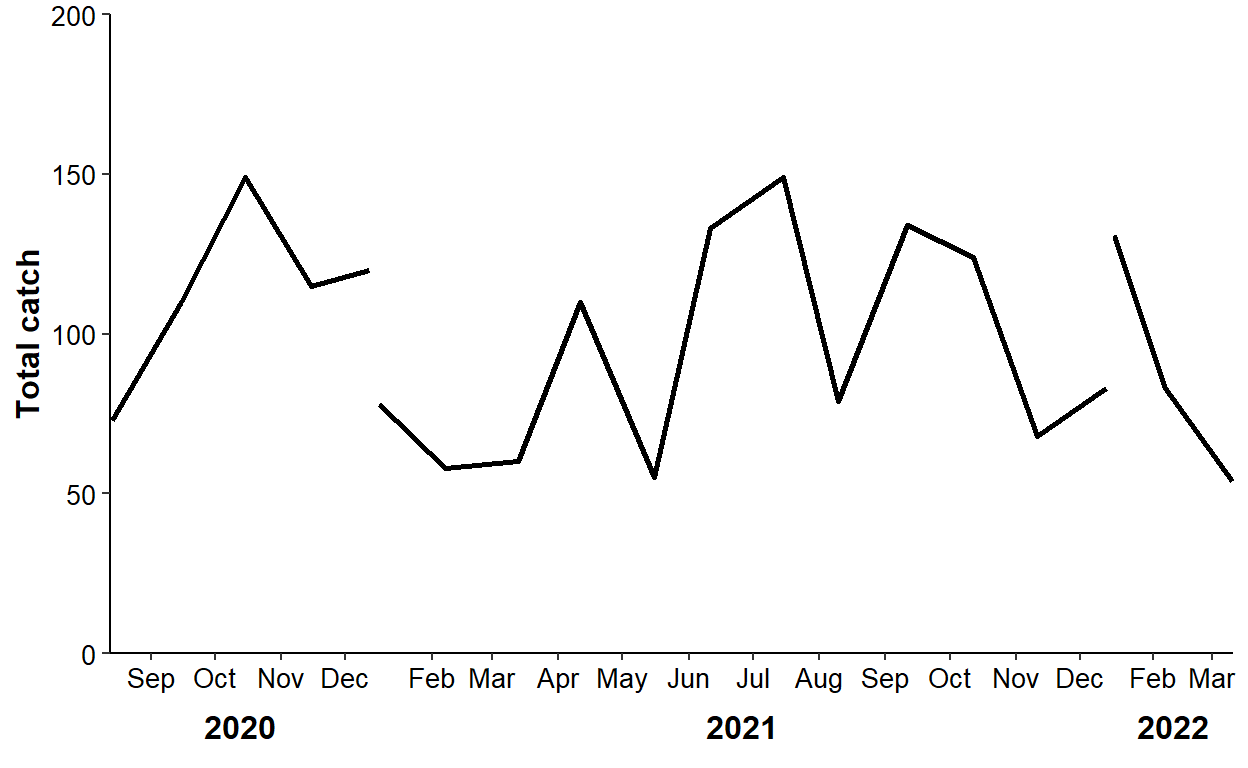

Option 3, however, will work for situations like this. For this example, segments should “cover” Sep-Dec for 2021, Jan-Dec for 2022, and Jan-Mar for 2023. Starting (in xstart) and ending (in xend) dates for these segments are put in a data frame below. A data frame of labels is then constructed from it similar to before, except that the label is the year extracted from the x-coordinate date.

x2lns <- data.frame(xstart=as.Date(c("20-Aug-2020","20-Dec-2020","20-Dec-2021"),
                                   format="%d-%B-%Y"),
                    xend=as.Date(c("15-Dec-2020","15-Dec-2021","15-Mar-2022"),
                                 format="%d-%B-%Y"))

x2lbls <- x2lns |>
  rowwise() |>
  summarize(x=mean(c(xstart,xend))) |>
  ungroup() |>
  mutate(lbl=year(x))

Segments and labels are then added as before.⁸

⁸ Note the use of coord_cartesian(), geom_segment(), geom_text(), and plot.margin=.

ggplot(data=dat2,mapping=aes(x=sample_date,y=catch)) +
  geom_line(linewidth=1) +
  scale_x_date(breaks=scales::breaks_width("month"),
               labels=scales::label_date("%b"),expand=expansion(mult=0.01)) +
  scale_y_continuous(name="Total catch",expand=expansion(mult=0)) +
  coord_cartesian(ylim=c(0,200),clip="off") +
  theme_classic() +
  theme(axis.title=element_text(size=12,face="bold"),
        axis.title.x=element_blank(),
        axis.text=element_text(size=10,color="black"),
        plot.margin=margin(t=1,l=1,b=2,r=1,unit="lines")) +
  geom_segment(data=x2lns,mapping=aes(x=xstart,xend=xend),y=-18,yend=-18,
               linewidth=0.75) +
  geom_text(data=x2lbls,mapping=aes(x=x,label=lbl),y=-26,
            size=12/.pt,fontface="bold")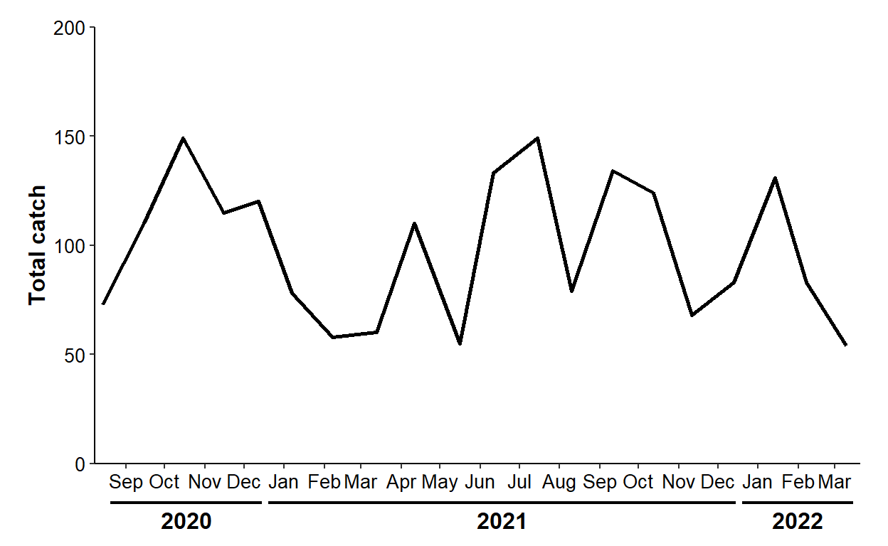

Example 4 - Histogram

In this example, I use data on female Walleye captured from location “2” in Lake Erie in 2010.

Code

data(WalleyeErie2,package="FSAdata")
waedat <- WalleyeErie2 |>
  filter(loc==2,year==2010,sex=="female")
FSA::headtail(waedat)

#R|        setID loc grid year  tl    w    sex    mat age
#R|  1   2010019   2 1005 2010 642 3138 female mature   7
#R|  2   2010019   2 1005 2010 686 3360 female mature   7
#R|  3   2010019   2 1005 2010 685 3489 female mature  11
#R|  919 2010058   2 1230 2010 715 4169 female mature  10
#R|  920 2010058   2 1230 2010 549 1853 female mature   3
#R|  921 2010058   2 1230 2010 596 2432 female mature   7

Suppose we want to make a simple length frequency histogram like that below,⁹ but with Gabelhouse length categories (“stock”, “quality”, etc.) listed below the lengths but above the title on the x-axis.¹⁰

⁹ See this post about making length frequency histograms in ggplot2.

¹⁰ There are probably better ways to create these labels, but this works as a demonstration of the secondary x-axis.

ggplot(data=waedat,mapping=aes(x=tl)) +
  geom_histogram(binwidth=10,boundary=0,closed="left",
                 color="black",fill="gray50") +
  scale_y_continuous(name="Frequency",expand=expansion(mult=c(0,0.025))) +
  scale_x_continuous(name="Total Length (mm)",breaks=scales::breaks_width(50)) +
  theme_bw() +
  theme(axis.text=element_text(color="black"))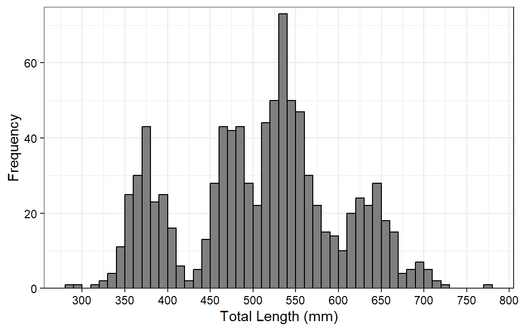

The values for the Gabelhouse length categories are obtained from psdVal() in FSA.

( waepsd <- FSA::psdVal("Walleye",incl.zero=FALSE) )

#R|      stock   quality preferred memorable    trophy 
#R|        250       380       510       630       760

These values are used to make the endpoints of the segment lines, noting that each stops 2 mm before the next segment starts so as to provide a visible break in the segments. A data frame of labels was created as above, except that the text for the labels came from the names provided with psdVal(). Also note that 810 (i.e., the end of the x-axis) was appended to the segment ends so that the “trophy” segment would have an end point.

x2lns <- data.frame(xstart=waepsd,xend=c(waepsd[-1]-2,810))
x2lns

#R|            xstart xend
#R|  stock        250  378
#R|  quality      380  508
#R|  preferred    510  628
#R|  memorable    630  758
#R|  trophy       760  810

x2lbls <- x2lns |>
  rowwise() |>
  summarize(x=mean(c(xstart,xend))) |>
  ungroup() |>
  mutate(lbl=names(waepsd))
x2lbls

#R|  # A tibble: 5 × 2
#R|        x lbl      
#R|    <dbl> <chr>    
#R|  1   314 stock    
#R|  2   444 quality  
#R|  3   569 preferred
#R|  4   694 memorable
#R|  5   785 trophy

Making room for the secondary labels is a little different here because the x-axis title is maintained. Thus, instead of changing plot.margin() as above, more space is added by increasing the top margin of the x-axis title with axis.title.x=.

ggplot(data=waedat,mapping=aes(x=tl)) +
  geom_histogram(binwidth=10,boundary=0,closed="left",
                 color="black",fill="gray50") +
  scale_y_continuous(name="Frequency",expand=expansion(mult=c(0,0.025))) +
  scale_x_continuous(name="Total Length (mm)",breaks=scales::breaks_width(50),
                     expand=expansion(mult=0.025)) +
  theme_bw() +
  theme(axis.text=element_text(color="black"),
        axis.title.x=element_text(margin=margin(t=3,unit="lines")))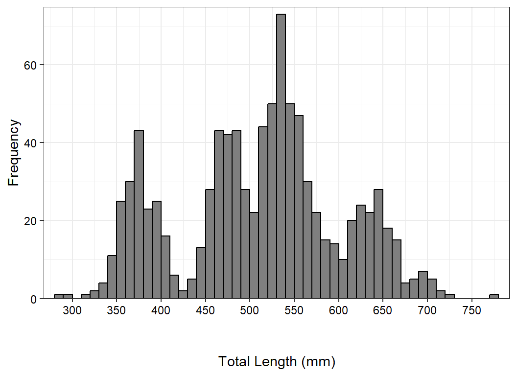

This space is then filled with the secondary axis labels as before.

ggplot(data=waedat,mapping=aes(x=tl)) +
  geom_histogram(binwidth=10,boundary=0,closed="left",
                 color="black",fill="gray50") +
  scale_y_continuous(name="Frequency",expand=expansion(mult=c(0,0.025))) +
  scale_x_continuous(name="Total Length (mm)",breaks=scales::breaks_width(50),
                     expand=expansion(mult=0.025)) +
  theme_bw() +
  theme(axis.text=element_text(color="black"),
        axis.title.x=element_text(margin=margin(t=3,unit="lines"))) +
  coord_cartesian(xlim=c(250,800),clip="off") +
  geom_segment(data=x2lns,mapping=aes(x=xstart,xend=xend),y=-7,yend=-7,
               linewidth=0.75) +
  geom_text(data=x2lbls,mapping=aes(x=x,label=lbl),y=-10,
            size=11/.pt)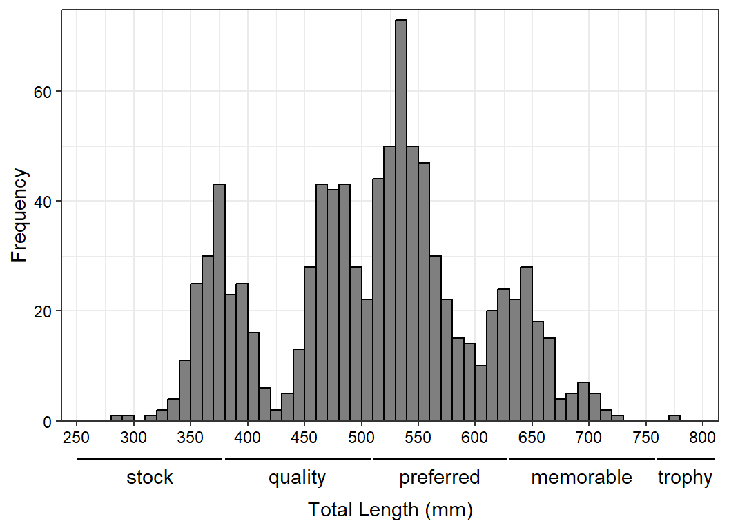

Further Thoughts

Option 3 provides a great deal of flexibility. For example, suppose for the length frequency histogram that the segments are separated with vertical lines rather than breaks. To accomplish this, the 2 mm spacing in the segments data frame must be removed.

x2lns <- data.frame(xstart=waepsd,xend=c(waepsd[-1],810))

x2lbls <- x2lns |>
  rowwise() |>
  summarize(x=mean(c(xstart,xend))) |>
  ungroup() |>
  mutate(lbl=names(waepsd))

Then, for the segments, arrows are added at the beginning, but with a 90^o angle so that they look like vertical lines.¹¹

¹¹ “Arrows” only at the beginning of the segments will make the last “trophy” segment appear open-ended, as it should.

ggplot(data=waedat,mapping=aes(x=tl)) +
  geom_histogram(binwidth=10,boundary=0,closed="left",
                 color="black",fill="gray50") +
  scale_y_continuous(name="Frequency",expand=expansion(mult=c(0,0.025))) +
  scale_x_continuous(name="Total Length (mm)",breaks=scales::breaks_width(50),
                     expand=expansion(mult=0.025)) +
  theme_bw() +
  theme(axis.text=element_text(color="black"),
        axis.title.x=element_text(margin=margin(t=3,unit="lines"))) +
  coord_cartesian(xlim=c(250,800),clip="off") +
  geom_segment(data=x2lns,mapping=aes(x=xstart,xend=xend),y=-7,yend=-7,
               linewidth=0.75,
               arrow=arrow(ends="first",type="closed",angle=90,length=unit(4,"pt"))) +
  geom_text(data=x2lbls,mapping=aes(x=x,label=lbl),y=-10,
            size=11/.pt)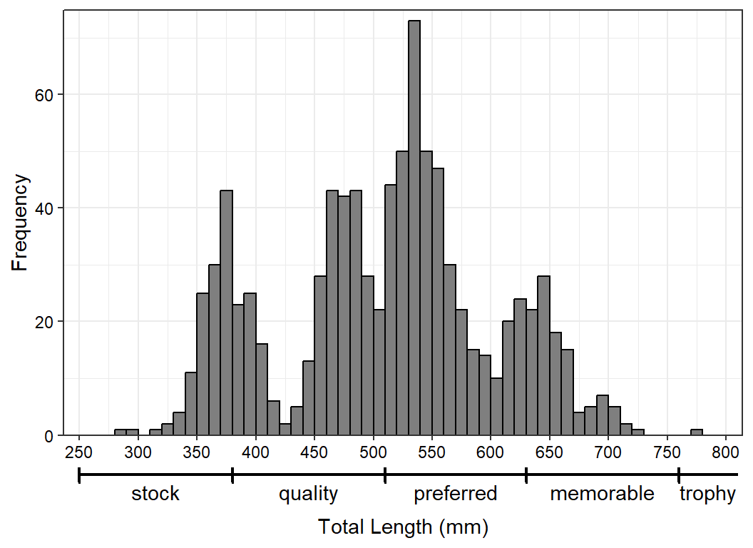

As another example, geom_rect() with judicious choices for ymin= and ymax= can be used to provide more options for the secondary axis labels.¹²

¹² Note here that data= and mapping= had to moved out of ggplot() and put into geom_histogram() for this to work.

ggplot() +
  geom_histogram(data=waedat,mapping=aes(x=tl),
                 binwidth=10,boundary=0,closed="left",
                 color="black",fill="gray50") +
  scale_y_continuous(name="Frequency",expand=expansion(mult=c(0,0.025))) +
  scale_x_continuous(name="Total Length (mm)",breaks=scales::breaks_width(50),
                     expand=expansion(mult=0.025)) +
  theme_bw() +
  theme(axis.text=element_text(color="black"),
        axis.title.x=element_text(margin=margin(t=3,unit="lines"))) +
  coord_cartesian(xlim=c(250,800),clip="off") +
  geom_rect(data=x2lns,mapping=aes(xmin=xstart,xmax=xend),ymin=-12,ymax=-6,
               fill="gray70",color="gray30") +
  geom_text(data=x2lbls,mapping=aes(x=x,label=lbl),y=-8.75,
            size=11/.pt)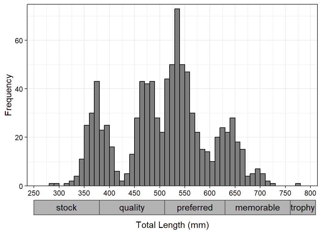

Reuse

https://creativecommons.org/licenses/by/4.0/

Citation

BibTeX citation:

@online{h. ogle2023,
  author = {H. Ogle, Derek},
  title = {Nested {X-Axis} {Labels}},
  date = {2023-03-30},
  url = {https://fishr-core-team.github.io/fishR//blog/posts/2023-3-30_Nested_xaxis},
  langid = {en}
}

For attribution, please cite this work as:

H. Ogle, D. 2023, March 30. Nested X-Axis Labels. https://fishr-core-team.github.io/fishR//blog/posts/2023-3-30_Nested_xaxis.