library(tidyverse)  # for dplyr, ggplot2 packages
library(scales)     # for breaks_width()
library(ggh4x) # for minor tick functionality and facetted_pos_scales()Introduction
Rook et al. (2022) analyzed historical data to answer the question of how many ciscoes are needed for stocking in the Laurentian Great Lakes. Their Figure 2 shows the commercial harvest of Cisco (Coregonus artedii) and deepwater ciscoes (Coregonus spp.) in the five main Great Lakes and St. Clair. The main point of their figure was to demonstrate the great reduction in harvest of these species by the 1970s.
The following packages are loaded for use below.
Get Data
Rook et al. (2022) did not provide data for Figure 2, but they did provide a reference that linked to a database maintained by the Great Lakes Fishery Commission that contained an Excel spreadsheet with harvest data for each lake (in separate sheets) for ALL species. Below each sheet is read into into its own data frame and reduced to just the variables needed for this post,1
1 Note that the total harvest variable was inconsistently named across sheets.
eri <- readxl::read_excel("commercial.xlsx",sheet="Erie") |>
  select(Year,Lake,Species,Total=`Grand Total`)
ont <- readxl::read_excel("commercial.xlsx",sheet="Ontario") |>
  select(Year,Lake,Species,Total=`Grand Totals`) #!!
hur <- readxl::read_excel("commercial.xlsx",sheet="Huron") |>
  select(Year,Lake,Species,Total=`Grand Total`)
sup <- readxl::read_excel("commercial.xlsx",sheet="Superior") |>
  select(Year,Lake,Species,Total=`Grand Total`)
mic <- readxl::read_excel("commercial.xlsx",sheet="Michigan") |>
  select(Year,Lake,Species,Total=`U.S. Total`) #!!
stc <- readxl::read_excel("commercial.xlsx",sheet="St. Clair") |>
  select(Year,Lake,Species,Total=`Grand Total`)
The individual data frames are then row-bound (i.e., stacked) together, the Lake variable is moved to the first column, and the data are sorted by Lake, Year, and Species.2
2 Moving Lake and sorting was for personal aesthetics.
dat <- bind_rows(eri,ont,hur,sup,mic,stc) |>
  relocate(Lake) |>
  arrange(Lake,Year,Species)
I examined the names in Species so that I could restrict the data frame to Cisco and deepwater ciscoes.
unique(dat$Species)#R| [1] "Cisco" "Lake Whitefish"
#R| [3] "Walleye and Blue Pike" "Northern Pike"
#R| [5] "Lake Sturgeon" "Blue Pike"
#R| [7] "Channel Catfish and Bullheads" "Sauger"
#R| [9] "Walleye" "Yellow Perch"
#R| [11] "Suckers" "Carp"
#R| [13] "Burbot" "Freshwater Drum"
#R| [15] "White Bass" "Bullheads"
#R| [17] "Channel Catfish" "Goldfish"
#R| [19] "Rainbow Smelt" "Pacific Salmon"
#R| [21] "Bowfin" "Buffalo"
#R| [23] "Gizzard Shad" "Lake Trout"
#R| [25] "Minnows" "Quillback"
#R| [27] "Rock Bass" "Sunfish"
#R| [29] "White Perch" "American Eel"
#R| [31] "Crappie" "Channel catfish"
#R| [33] "Gar" "Round Whitefish"
#R| [35] "Cisco and Chubs" "Chubs"
#R| [37] "Pacific salmon" "Crappies"
#R| [39] "Cisco and Chub" "Alewife"
#R| [41] "Coho Salmon" "Chinook Salmon"
#R| [43] "Amercian Eel" "White bass"
#R| [45] "Herring" "Smallmouth Bass"
#R| [47] "Bullhead" "Drum"
#R| [49] "Rock Bass and Crappie" "Sheepshead"
#R| [51] "Cisco and chubs" "Lake Trout - siscowet"This was a little messier than I had hoped. First, “Cisco” are sometimes called “Herring”, so both of these “species” must be retained. Deepwater ciscoes are often called “chubs”, so this “species” must be retained. However, there were also “species” called various versions of “Cisco and Chubs”, all of which need to be retained. A new data frame is created below with just these “species” and, to match Rook et al. (2022), only years of 1880 to 2015 (inclusive) were retained.
cdat <- dat |>
  filter(Species %in% c("Cisco","Chubs","Cisco and Chubs",
                        "Cisco and chubs","Cisco and chub","Herring")) |>
  filter(Year>=1880,Year<=2015)
For what it is worth, it seems that the use of “Cisco and chubs” for Lake Superior should be corrected in the database, and “Herring” for Lake St. Clair should be changed to “Cisco.”
xtabs(~Lake+Species,data=cdat)#R| Species
#R| Lake Chubs Cisco Cisco and chubs Cisco and Chubs Herring
#R| Erie 0 102 0 0 0
#R| Huron 113 113 0 29 0
#R| Michigan 126 107 0 0 0
#R| Ontario 64 64 0 72 0
#R| Saint Clair 0 0 0 0 39
#R| Superior 123 136 61 0 0Figure 2 ultimately lumps all of these “species” together within each year and lake combination. For example, in the portion of cdat below the two entries for 2015 for Lake Superior should be combined to form one entry.
FSA::headtail(cdat)#R| Lake Year Species Total
#R| 1 Erie 1880 Cisco 882.000
#R| 2 Erie 1881 Cisco 1868.000
#R| 3 Erie 1882 Cisco 2008.000
#R| 1147 Superior 2014 Cisco 1587.571
#R| 1148 Superior 2015 Chubs 87.638
#R| 1149 Superior 2015 Cisco 1983.159Additionally, it is important to note that some Total values are missing (coded as NA). Thus, an adjustment will be made below for these NAs when summing to make a composite harvest value for each year and lake.
any(is.na(cdat$Total))#R| [1] TRUEA new data frame is created from the data frame above that groups the data by Year within Lake and then sums the Total harvest for all “species” in each lake-year combination into a variable called Coregonids. na.rm=TRUE is used in sum to ignore the NAs.3 The data frame is ungroup()ed before moving on.
3 Otherwise, any sum with an NA value will return NA.
cdat2 <- cdat |>
  group_by(Lake,Year) |>
  summarize(Coregonids=sum(Total,na.rm=TRUE)) |>
  ungroup()
FSA::peek(cdat2,n=10)
#R| Lake Year Coregonids
#R| 1 Erie 1880 882.000
#R| 75 Erie 1954 381.000
#R| 150 Huron 1927 7694.000
#R| 225 Huron 2002 118.622
#R| 300 Michigan 1951 18675.000
#R| 375 Ontario 1890 3084.000
#R| 450 Ontario 1965 31.000
#R| 525 Saint Clair 1904 27.000
#R| 600 Superior 1940 36879.000
#R| 675 Superior 2015 2070.797It was not obvious to me from the Great Lakes Fisheries Commission website what the units are for these harvest data. In comparison to Rook et al. (2022) they appear to be hundreds of thousands of pounds. Rook et al. (2022) plotted millions of kgs so I first convert Coregonids to kg and then divide by 1000 to get to millions of kgs.
cdat2 <- cdat2 |>
  mutate(Coregonids=Coregonids*0.45359237,
         Coregonids=Coregonids/1000)
An issue that happens regularly with these type of data with this type of plot occurs when the data does not have continuous years. For example, suppose that harvest was recorded for 1900 and 1902 but not 1901. If 1901 is completely excluded from the data, rather than being entered as an NA, then the line in the plot will connect directly from 1900 to 1902 suggesting, if the reader is not paying close attention, that a value exists in 1901. You can see many unconnected dots in Figure 2 of Rook et al. (2022) that illustrate how these missing data should be handled.
With these data, it appears that the years are contiguous within each lake except for Lake Erie, but only complete (for 1880-2015) for lakes Huron, Ontario, and Superior.
cdat2 |>
  group_by(Lake) |>
  summarize(numYrs=n(),
            minYr=min(Year),
            maxYr=max(Year),
            rngYr=maxYr-minYr+1,
            contigYr=ifelse(rngYr==numYrs,"Yes","No"),
            compltYr=ifelse(numYrs==(2015-1880+1),"Yes","No"))
#R| # A tibble: 6 × 7
#R| Lake numYrs minYr maxYr rngYr contigYr compltYr
#R| <chr> <int> <dbl> <dbl> <dbl> <chr> <chr>
#R| 1 Erie 102 1880 2015 136 No No
#R| 2 Huron 136 1880 2015 136 Yes Yes
#R| 3 Michigan 126 1890 2015 126 Yes No
#R| 4 Ontario 136 1880 2015 136 Yes Yes
#R| 5 Saint Clair 39 1880 1918 39 Yes No
#R| 6 Superior 136 1880 2015 136 Yes YesThe issue with Lake Erie appears to be many years of missing data from 1977 to 2012.
tmp <- cdat2 |>
  filter(Lake=="Erie")
tmp$Year
#R| [1] 1880 1881 1882 1883 1884 1885 1886 1887 1888 1889 1890 1891 1892 1893 1894
#R| [16] 1895 1896 1897 1898 1899 1900 1901 1902 1903 1904 1905 1906 1907 1908 1909
#R| [31] 1910 1911 1912 1913 1914 1915 1916 1917 1918 1919 1920 1921 1922 1923 1924
#R| [46] 1925 1926 1927 1928 1929 1930 1931 1932 1933 1934 1935 1936 1937 1938 1939
#R| [61] 1940 1941 1942 1943 1944 1945 1946 1947 1948 1949 1950 1951 1952 1953 1954
#R| [76] 1955 1956 1957 1958 1959 1960 1961 1962 1963 1964 1965 1966 1967 1968 1969
#R| [91] 1970 1971 1972 1973 1974 1975 1976 1977 2012 2013 2014 2015To make sure that the data are contiguous and cover the range of years, expand_grid() was used first to create a temporary data frame with each year from 1880 to 2015 (inclusive) listed for each lake.
tmp <- expand_grid(Lake=unique(cdat2$Lake),
                   Year=min(cdat2$Year):max(cdat2$Year))

FSA::headtail(tmp)
#R| Lake Year
#R| 1 Erie 1880
#R| 2 Erie 1881
#R| 3 Erie 1882
#R| 814 Superior 2013
#R| 815 Superior 2014
#R| 816 Superior 2015This data frame was left_join() with cdat2, using both Lake and Year as the id variables, so that every lake-year combination in tmp was matched with a Total from the corresponding lake-year combination in cdat2 or an NA if the lake-year combination did not exist in cdat2.
cdat3 <- left_join(tmp,cdat2,by=c("Lake","Year"))Now the years are contiguous and complete for each lake.
cdat3 |>
  group_by(Lake) |>
  summarize(numYrs=n(),
            minYr=min(Year),
            maxYr=max(Year),
            rngYr=maxYr-minYr+1,
            contigYr=ifelse(rngYr==numYrs,"Yes","No"),
            compltYr=ifelse(numYrs==(2015-1880+1),"Yes","No"))
#R| # A tibble: 6 × 7
#R| Lake numYrs minYr maxYr rngYr contigYr compltYr
#R| <chr> <int> <dbl> <dbl> <dbl> <chr> <chr>
#R| 1 Erie 136 1880 2015 136 Yes Yes
#R| 2 Huron 136 1880 2015 136 Yes Yes
#R| 3 Michigan 136 1880 2015 136 Yes Yes
#R| 4 Ontario 136 1880 2015 136 Yes Yes
#R| 5 Saint Clair 136 1880 2015 136 Yes Yes
#R| 6 Superior 136 1880 2015 136 Yes YesFinally, Lake is made a factor with the levels specified so that the lakes will be ordered as in Figure 2 of Rook et al. (2022)
cdat3 <- cdat3 |>
  mutate(Lake=factor(Lake,levels=c("Superior","Huron","Michigan",
                                   "Erie","Ontario","Saint Clair")))
As will be shown further below, these data do not appear to be exactly the data used in Rook et al. (2022). One of several issues that is evident is that their Figure 2 shows many years of missing data (i.e., points not connected with lines) early in the time series for most lakes, whereas there were few missing years in my data frame. I suspected that Rook et al. (2022) may have coded a harvest of 0 as NA so, to explore this, I created a new variable called is0 that I will plot differently further below. I did this only to troubleshoot this data issue, not as part of recreating their Figure 2.
cdat3 <- cdat3 |>
  mutate(is0=Coregonids==0)
Recreating Figure 2
The ggplot2 theme was set to theme_classic() but with modifications to remove the background for facet labels, increase the spacing between facets, remove the legend,4 make tick marks slightly longer, and make minor tick marks 50% as big as the major tick marks.5
4 The only reason there is a legend is because I am going to highlight points where the harvest was 0.
5 This requires the ggh4x package attached above.
theme_set(
  theme_classic() +
    theme(strip.background=element_blank(),
          panel.spacing=unit(5,"mm"),
          legend.position="none",
          axis.ticks.length.x=unit(5,units="pt"),
          ggh4x.axis.ticks.length.minor=rel(0.5)))
I could not find a simple way to have minor ticks, ticks that crossed the axes, and differing y-axis limits for each facet as used in Figure 2 of Rook et al. (2022). Thus, I opted to not have ticks that crossed the axes.
A basic plot is constructed below from cdat3 with Year mapped to the x-axis and Coregonids mapped to the y-axis with geom_line() and geom_point() to plot the line with points. facet_wrap() was used to separate the plots by lake. In facet_wrap() both scales were “freed” because the y-axes need to change by lake and, though the x-axes don’t differ by lake, freeing the x-axes will force an x-axis to be shown for each lake as in Rook et al. (2022). is0 is mapped to a color in geom_point(), and the colors are defined in scale_color_manual(), to show years that had 0 harvest as red.&(Again, this is not in Rook et al. 2022, but I was trying to better understand why my data appeared different than theirs.)
ggplot(data=cdat3,mapping=aes(x=Year,y=Coregonids)) +
  geom_line() +
  geom_point(mapping=aes(color=is0),size=1) +
  scale_color_manual(values=c("FALSE"="black","TRUE"="red")) +
  facet_wrap(vars(Lake),scales="free",ncol=2)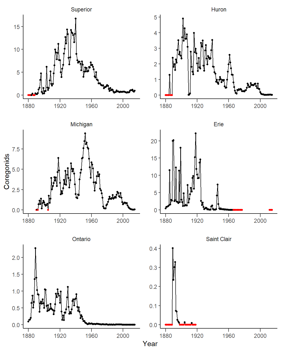
Some challenges remain to try to match Figure 2 in Rook et al. (2022). First, the x-axes need to be bound from 1880 to 2020, the tick mark labels need to be shown at intervals of 20 years, and minor ticks need to be shown at 5 year intervals. The axes bounds are set with limits=, major (i.e., labeled) breaks are set with breaks= using breaks_width(),6 and minor breaks are set with minor_breaks= also using breaks_width().7 Note the use of guide= so that the minor breaks will be shown.
6 breaks_width() requires the scales package attached above.
7 As described in this post.
ggplot(data=cdat3,mapping=aes(x=Year,y=Coregonids)) +
  geom_line() +
  geom_point(mapping=aes(color=is0),size=1) +
  scale_x_continuous(limits=c(1880,2020),expand=expansion(mult=0),
                     breaks=breaks_width(20),
                     minor_breaks=breaks_width(5),guide="axis_minor") +
  scale_color_manual(values=c("FALSE"="black","TRUE"="red")) +
  facet_wrap(vars(Lake),scales="free",ncol=2)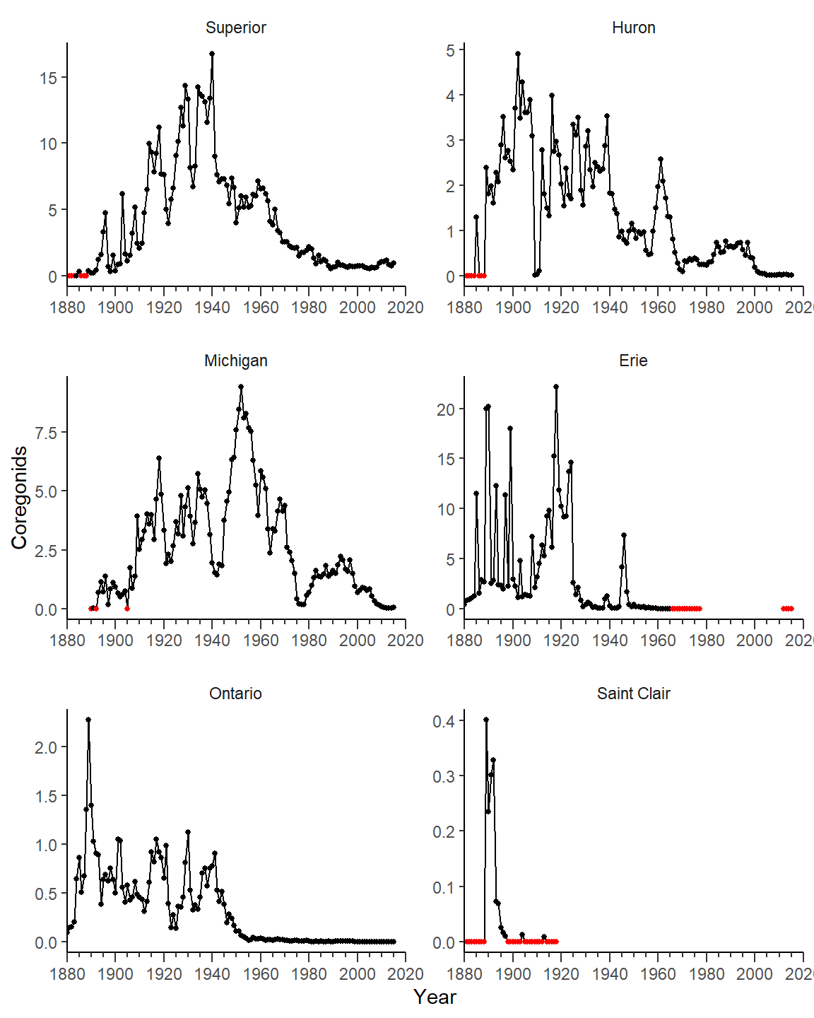
Now the y-axes need a different label and different upper limits, major tick labels, and minor ticks per facet/panel. All of these items may be adjusted on a per-facet basis with facetted_pos_scales() which is described in more detail in this post. For these purposes, y= in facetted_pos_scales() will receive a list with as many scale_y_continuous() items in it as facets (i.e., six). Each scale_y_continuous() item in this list will define the y-axis for a facet, ordered across rows and down columns. For example, the first scale_y_continuous() item is for Lake Superior and the last is for Lake St. Clair. Note that the name for the y-axis only needs to be defined in the first scale_y_continous() item in the list.
syc <- list(
  scale_y_continuous(name="Commercial Harvest (millions of kg)",
                     limits=c(0,20),expand=expansion(mult=0),
                     breaks=breaks_width(5),minor_breaks=breaks_width(5/5),
                     guide="axis_minor"),
  scale_y_continuous(limits=c(0,5),expand=expansion(mult=0),
                     breaks=breaks_width(1),minor_breaks=breaks_width(1/5),
                     guide="axis_minor"),
  scale_y_continuous(limits=c(0,15),expand=expansion(mult=0),
                     breaks=breaks_width(5),minor_breaks=breaks_width(5/5),
                     guide="axis_minor"),
  scale_y_continuous(limits=c(0,25),expand=expansion(mult=0),
                     breaks=breaks_width(5),minor_breaks=breaks_width(5/5),
                     guide="axis_minor"),
  scale_y_continuous(limits=c(0,2.5),expand=expansion(mult=0),
                     breaks=breaks_width(0.5),minor_breaks=breaks_width(0.5/5),
                     guide="axis_minor"),
  scale_y_continuous(limits=c(0,0.5),expand=expansion(mult=0),
                     breaks=breaks_width(0.1),minor_breaks=breaks_width(0.1/5),
                     guide="axis_minor")
  )
For convenience the list was entered into an object above and given to facetted_pos_scale() below.
ggplot(data=cdat3,mapping=aes(x=Year,y=Coregonids)) +
  geom_line() +
  geom_point(mapping=aes(color=is0),size=1) +
  scale_x_continuous(limits=c(1880,2020),expand=expansion(mult=0),
                     breaks=breaks_width(20),
                     minor_breaks=breaks_width(5),guide="axis_minor") +
  scale_color_manual(values=c("FALSE"="black","TRUE"="red")) +
  facet_wrap(vars(Lake),scales="free",ncol=2) +
  facetted_pos_scales(y=syc)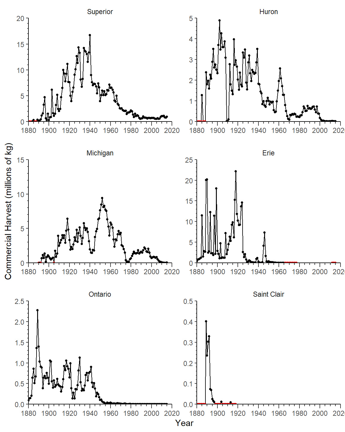
Finally, Rook et al. (2022) placed the lake labels in the upper-right corner of each facet rather than centered above each facet. To accomplish this use geom_text() with Lake mapped to a label. This will, by default, print the lake name for each facet over-and-over for as many rows as there are for the lake in the data frame. To eliminate these overlapping labels, include check_overlap=TRUE. The label position was set to the maximum x and maximum y value for each facet by using both x=Inf and y=Inf. The label was then moved left (with vjust=) and down (with hjust=) as described in this post. The font size was reduced from the default slightly. Finally, the default facet labels must be removed by setting strip.text= to element_blank() in theme().
ggplot(data=cdat3,mapping=aes(x=Year,y=Coregonids)) +
  geom_line() +
  geom_point(mapping=aes(color=is0),size=1) +
  geom_text(mapping=aes(label=Lake),check_overlap=TRUE,size=3.5,
            x=Inf,y=Inf,vjust=1.2,hjust=1.2) +
  scale_x_continuous(limits=c(1880,2020),expand=expansion(mult=0),
                     breaks=breaks_width(20),
                     minor_breaks=breaks_width(5),guide="axis_minor") +
  scale_color_manual(values=c("FALSE"="black","TRUE"="red")) +
  facet_wrap(vars(Lake),scales="free",ncol=2) +
  facetted_pos_scales(y=syc) +
  theme(strip.text=element_blank())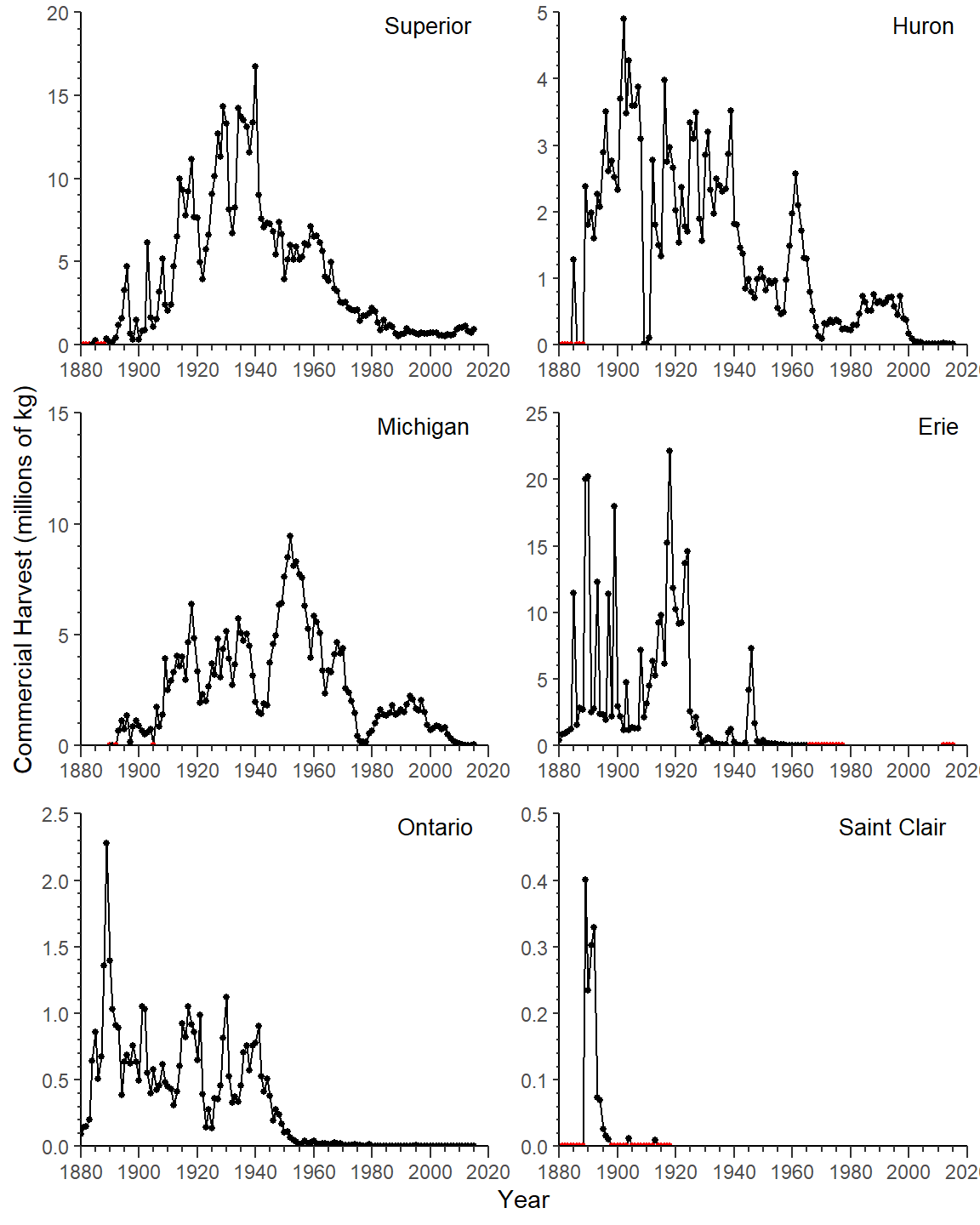
This largely recreates Figure 2 in Rook et al. (2022) with the exceptions of (a) tick marks that do not cross the axes and (b) discrepancies in the data used.
References
Rook, B. J., M. J. Hansen, and C. R. Bronte. 2022. How many Ciscoes are needed for stocking in the Laurentian Great Lakes? Journal of Fish and Wildlife Management 13(1):28–49.
Reuse
Citation
BibTeX citation:
@online{h._ogle2023,
  author = {H. Ogle, Derek},
  title = {Rook Et Al. (2022) {Cisco} {Harvest} {Figure}},
  date = {2023-03-17},
  url = {https://fishr-core-team.github.io/fishR/blog/posts/2023-3-18-Rooketal2022_CiscoHarvest/},
  langid = {en}
}
For attribution, please cite this work as:
H. Ogle, D. 2023, March 17. Rook et al. (2022) Cisco Harvest Figure. https://fishr-core-team.github.io/fishR/blog/posts/2023-3-18-Rooketal2022_CiscoHarvest/.