library(FSA)     # for vbFuns(), vbStarts(), headtail()
library(dplyr)   # for filter(), mutate()
library(ggplot2)
theme_set(theme_bw())
Note
The following packages are loaded for use below. One function from investr is also used but the whole package is not loaded here. The data are also from FSAdata, which is not loaded below. I also set the default ggplot theme to theme_bw() for a classic “black-and-white” plot (rather than the default plot with a gray background).
Introduction
The most common questions that I receive through the fishR website are related to fitting a von Bertalanffy growth function (VBGF) to data and viewing the results. In this post, I briefly demonstrate how to fit a VBGF to a single group of data and then provide several options for how to view the fit of the function to those data.
I will use lengths and ages of Lake Erie Walleye (Sander vitreus) captured during October-November, 2003-2014 available in FSAdata package. These data formed many of the examples in Ogle et al. (2017). My primary interest here is in the tl (total length in mm) and age variables1. I focus on female Walleye from location “1” captured in 2014 in this example.2
1 See more details about the data.
2 For succinctness, I removed year and sex as they only had one category after filtering and three variables related to the location of capture.
data(WalleyeErie2,package="FSAdata")
wf14T <- WalleyeErie2 |>
  filter(year==2014,sex=="female",loc==1) |>
  select(-year,-sex,-setID,-loc,-grid)
headtail(wf14T)
#R| tl w mat age
#R| 1 445 737 immature 2
#R| 2 528 1571 mature 4
#R| 3 380 506 immature 1
#R| 323 488 1089 immature 2
#R| 324 521 1408 mature 3
#R| 325 565 1745 mature 3
Fitting the VBGF
Methods for fitting a von Bertalannfy growth function (VBGF) are detailed in Ogle (2016) and Ogle et al. (2017). Thus, this methodology will only be briefly explained here.
A function for the typical VBGF is constructed with vbFuns().3
3 Other parameterizations of the VBGF can be used with param= in vbFuns() as described in its documentation.
( vb <- vbFuns(param="Typical") )#R| function (t, Linf, K = NULL, t0 = NULL)
#R| {
#R| if (length(Linf) == 3) {
#R| K <- Linf[[2]]
#R| t0 <- Linf[[3]]
#R| Linf <- Linf[[1]]
#R| }
#R| Linf * (1 - exp(-K * (t - t0)))
#R| }
#R| <bytecode: 0x000001ece829d0a8>
#R| <environment: 0x000001ece82dbdb8>Some of the methods below use the fact that the three parameters of the typical VBGF (\(L_{\infty}\), \(K\), \(t_{0}\)) can be given to this function separately (in that order) or as a vector (still in that order). For example, both lines below can be used to predict the mean length for an age-3 fish with the given VBGF parameters.4
4 The parameters could be given in a different order but would need to be named; e.g., vb(3,t0=-0.5,K=0.3,Linf=300).
vb(3,300,0.3,-0.5)#R| [1] 195.0187tmp <- c(300,0.3,-0.5)
vb(3,tmp)#R| [1] 195.0187Reasonable starting values for the optimization algorithm may be obtained with vbStarts(), where the first argument is a formula of the form lengths~ages where lengths and ages are replaced with the actual variable names that contain the observed lengths and ages, respectively, and data= is set to the data frame that contains those variables.
( sv0 <- vbStarts(tl~age,data=wf14T) )#R| $Linf
#R| [1] 645.2099
#R|
#R| $K
#R| [1] 0.3482598
#R|
#R| $t0
#R| [1] -1.548925The nls() function is typically used to estimate parameters of the VBGF from observed data. The first argument is a formula that has lengths on the left-hand-side and the VBGF function created above on the right-hand-side. The VBGF function has the ages variable as its first argument and then Linf, K, and t0 as the remaining arguments (just as they appear here). Again, the data frame with the observed lengths and ages is given to data= and the starting values derived above are given to start=.
fit0 <- nls(tl~vb(age,Linf,K,t0),data=wf14T,start=sv0)The parameter estimates and confidence intervals are extracted from the saved nls() object with coef() and confint(), respectively.5 They are column-bound together here for aesthetic reasons.
5 This confint() requires the MASS package which is usually loaded automatically with base R.
cbind(Est=coef(fit0),confint(fit0))#R| Est 2.5% 97.5%
#R| Linf 648.208364 629.6754671 669.0341553
#R| K 0.361540 0.3223327 0.4043957
#R| t0 -1.283632 -1.4592315 -1.1207317
Model Fit Using stat_function()
Here all “layers” of the plot will use the same data; thus, data= and the aes()thetic mappings are defined in ggplot(). Observed lengths and ages are added to the plot with geom_point(). The points in Figure 1 were made slightly larger than the default (with size=) and also with a fairly low transparency value to handle considerable over-plotting. scale_y_continuous() and scale_x_continuous() control aspects of y- and x-axes, respectively – labels for axes are given in name=, minimum and maximum limits for the axis are in limits=, and specific major breaks for the axis are in breaks=.6 Finally, the fitted model line is added to the plot with stat_function() with the VBGF function created above in fun= and a list of arguments to this function in args=.7 In Figure 1 I made the model line a little wider than the default. Finally the theme() was modified to remove the minor grid lines from both axes.8
6 seq(0,700,100) makes a vector of numbers from 0 to 700 in increments of 100 and 0:11 makes a vector of integers from 0 to 11.
7 The usage here exploits the fact that all three parameters of the VBGF can be given in the first parameter argument, Linf=.
8 Thus the gridlines only appear for labelled axis breaks.
ggplot(data=wf14T,aes(x=age,y=tl)) +
  geom_point(size=2,alpha=0.1) +
  scale_y_continuous(name="Total Length (mm)",
                     limits=c(0,700),breaks=seq(0,700,100)) +
  scale_x_continuous(name="Age (years)",breaks=0:11) +
  stat_function(fun=vb,args=list(Linf=coef(fit0)),linewidth=1) +
  theme(panel.grid.minor=element_blank())
The model line can be displayed outside the range of observed ages by including minimum and maximum values in xlim= over which the function in fun= will be evaluated. In Figure 2 I add a dashed line for the model that includes evaluation at ages outside the observed range of ages (first stat_function()) and then plotted the model line for observed ages on top of that (second stat_function()). This gives the impression of using a dashed line only for the ages that would be extrapolated.9
9 I would usually change the axis expansion factors here to clean this plot up a bit.
ggplot(data=wf14T,aes(x=age,y=tl)) +
  geom_point(size=2,alpha=0.1) +
  scale_y_continuous(name="Total Length (mm)",limits=c(0,700)) +
  scale_x_continuous(name="Age (years)",breaks=0:11) +
  stat_function(fun=vb,args=list(Linf=coef(fit0)),
                xlim=c(-1,12),linewidth=1,linetype="dashed") +
  stat_function(fun=vb,args=list(Linf=coef(fit0)),linewidth=1) +
  theme(panel.grid.minor=element_blank())
Model Fit Using geom_smooth()
geom_smooth() can use nls() to fit the VBGF “behind the scenes” and then add the resultant model line to the plot. For this purpose geom_smooth() requires method="nls" and se=FALSE.10 In addition, arguments for fitting the VBGF required by nls() must be in a list given to methods.args=. Minimum required arguments for fitting the VBGF are the VBGF formula= and start=ing values as shown for nls() above. Figure 3 uses geom_smooth() in this way to reproduce Figure 1.
10 se=FALSE is required because this argument is not implemented in nls().
ggplot(data=wf14T,aes(x=age,y=tl)) +
  geom_point(size=2,alpha=0.1) +
  scale_y_continuous(name="Total Length (mm)",limits=c(0,700)) +
  scale_x_continuous(name="Age (years)",breaks=0:11) +
  geom_smooth(method="nls",se=FALSE,
              method.args=list(formula=y~vb(x,Linf,K,t0),start=sv0),
              color="black",linewidth=1) +
  theme(panel.grid.minor.x=element_blank())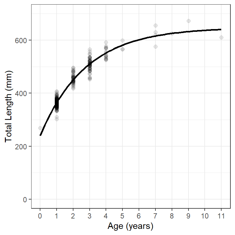
Model Fit from Predicted Values
Figure 1 and Figure 2 can also be constructed from lengths predicted at a variety of ages “outside” of any ggplot() layers. I find it easier when using this method to first create a vector of ages over which the fitted model will be evaluated is then constructed. In this case the ages extend beyond the observed range of ages. The seq()uence produced here will have 101 age values between -1 and 12.11
11 Use a larger value for length.out= to make the line produced further below more smooth.
ages <- seq(-1,12,length.out=101)The mean length at each of these ages is predicted with predict(), where the age vector just created is set equal to the name of the age variable in the nls() object inside of data.frame(). The vector of ages and predicted mean lengths are put into a data frame for plotting below.12
12 Here the data frame is called preds and it has two variables named age and fit.
preds <- data.frame(age=ages,
                    fit=predict(fit0,data.frame(age=ages)))
headtail(preds)
#R| age fit
#R| 1 -1.00 63.17547
#R| 2 -0.87 90.03596
#R| 3 -0.74 115.66322
#R| 99 11.74 642.36300
#R| 100 11.87 642.63138
#R| 101 12.00 642.88743
These predicted mean lengths-at-age are then used to add a fitted model line to a plot of observed lengths-at-age with geom_line(). However, because the observed and predicted data are in different data frames, the data= and mapped aes()thetics are declared within the appropriate geoms rather than within ggplot(). For example, geom_point() is used below to add the observed data to the plot and geom_line() is used below to add the modeled line. Note below that separate geom_line()s are used to show the modeled line over extrapolated and observed ages.13 The results in Figure 4 reproduce Figure 2.
13 Also note the use of filter() to reduce the predicted lengths-at-age to the observed ages.
ggplot() +
  geom_point(data=wf14T,aes(x=age,y=tl),size=2,alpha=0.1) +
  geom_line(data=preds,aes(x=age,y=fit),linewidth=1,linetype="dashed") +
  geom_line(data=filter(preds,age>=0,age<=11),aes(x=age,y=fit),linewidth=1) +
  scale_y_continuous(name="Total Length (mm)",limits=c(0,700)) +
  scale_x_continuous(name="Age (years)",breaks=0:11) +
  theme(panel.grid.minor=element_blank())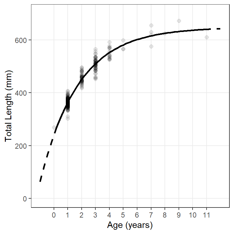
Model Fit with Confidence Band
The main reason for introducing the idea of constructing a graphic from predicted values is that it allows for the opportunity to add confidence and prediction bands around the fitted model line (Figure 5).
Creation of this plot requires modifying the data frame of predicted mean lengths at age with confidence (or prediction) intervals for the mean length at each age. As mentioned previously, constructing these intervals is not straightforward with non-linear models. However, confidence (or prediction) intervals can be estimated with Taylor series approximations as implemented in predFit() of investr.14 predFit() requires the saved nls() object as its first argument, a data frame of ages over which to make predictions as the second argument, and either interval="confidence" for confidence intervals or interval="prediction" for prediction intervals.
14 Use of :: here allows predFit() from investr to be used without loading all of investr.
preds <- data.frame(age=ages,
                    investr::predFit(fit0,data.frame(age=ages),
                                     interval="confidence"))
headtail(preds)
#R| age fit lwr upr
#R| 1 -1.00 63.17547 32.40761 93.94334
#R| 2 -0.87 90.03596 62.76575 117.30618
#R| 3 -0.74 115.66322 91.59342 139.73301
#R| 99 11.74 642.36300 625.59243 659.13357
#R| 100 11.87 642.63138 625.76065 659.50210
#R| 101 12.00 642.88743 625.91982 659.85504A confidence band for mean lengths at age is added to the plot with geom_ribbon() where the lower part of the ribbon is at the lower confidence values (i.e., ymin=lwr) and the upper part is at the upper confidence value (i.e., ymax=upr).15 fill= gives the color of the enclosed ribbon.
15 Add geom_ribbon() first so that it is behind the points and model lines.
ggplot() +
  geom_ribbon(data=preds,aes(x=age,ymin=lwr,ymax=upr),fill="gray80") +
  geom_point(data=wf14T,aes(y=tl,x=age),size=2,alpha=0.1) +
  geom_line(data=preds,aes(x=age,y=fit),linewidth=1,linetype="dashed") +
  geom_line(data=filter(preds,age>=0,age<=11),aes(x=age,y=fit),linewidth=1) +
  scale_y_continuous(name="Total Length (mm)",limits=c(0,700)) +
  scale_x_continuous(name="Age (years)",breaks=0:11) +
  theme(panel.grid.minor=element_blank())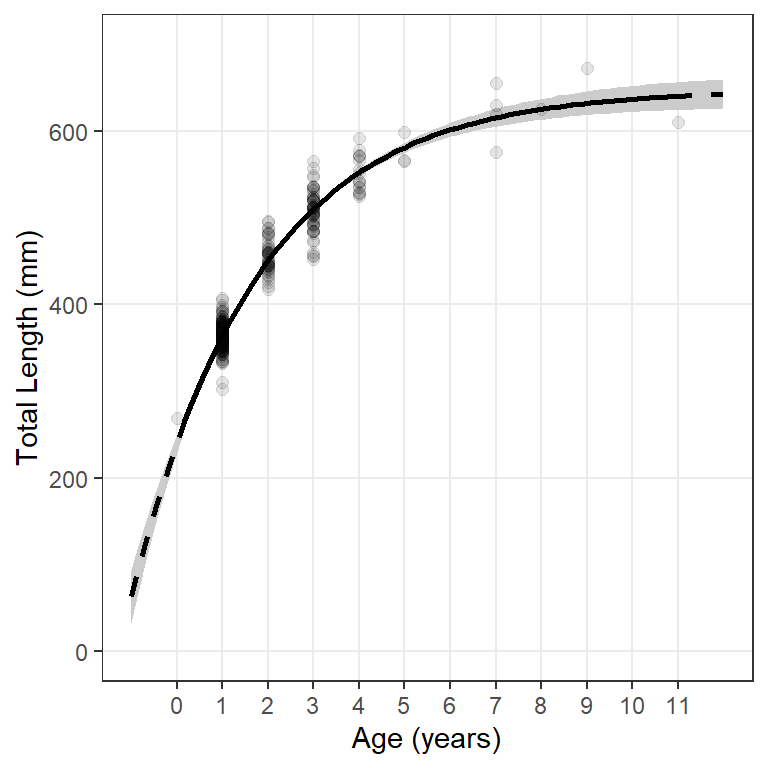
Add Equation to Plot
The following function can be used to extract the model coefficients from an nls() object and place them into a “plotmath” format to be added to the ggplot graph.
makeVBEqnLabel <- function(fit,digits=c(1,3,3)) {
  # Isolate coefficients (and control decimals)
  cfs <- coef(fit)
  Linf <- formatC(cfs[["Linf"]],format="f",digits=digits[1])
  K <- formatC(cfs[["K"]],format="f",digits=digits[2])
  # Handle t0 differently because of minus in the equation
  t0 <- cfs[["t0"]]
  sgn <- ifelse(t0<0,"+","-")
  t0 <- formatC(abs(t0),format="f",digits=digits[3])
  # Put together and return
  paste0("TL=='",Linf,"'~bgroup('[',1-e^{-'",K,"'~(age",sgn,"'",t0,"')},']')")
}
Note
The function above was modified on 14-Jun-23 to correct an issue with plotmath dropping trailing zeroes in the rounded coefficient values. For example a K of 0.250 would be printed as 0.25 when the string returned from makeVBEqnLabel() was parsed in annotate() below. The correction follows the suggestion in this StackOverflow post.
The object returned from this function can be added to the ggplot graph with annotate() as shown below.16
16 The x=, y=, hjust=, and vjust= arguments are used to position and justify the text and may take some trial-and-error to get what you want.
ggplot() +
  geom_ribbon(data=preds,aes(x=age,ymin=lwr,ymax=upr),fill="gray80") +
  geom_point(data=wf14T,aes(y=tl,x=age),size=2,alpha=0.1) +
  geom_line(data=preds,aes(x=age,y=fit),linewidth=1,linetype="dashed") +
  geom_line(data=filter(preds,age>=0,age<=11),aes(x=age,y=fit),linewidth=1) +
  scale_y_continuous(name="Total Length (mm)",limits=c(0,700)) +
  scale_x_continuous(name="Age (years)",breaks=0:11) +
  theme(panel.grid.minor=element_blank()) +
  annotate(geom="text",label=makeVBEqnLabel(fit0),parse=TRUE,
           size=4,x=Inf,y=-Inf,hjust=1.1,vjust=-0.5)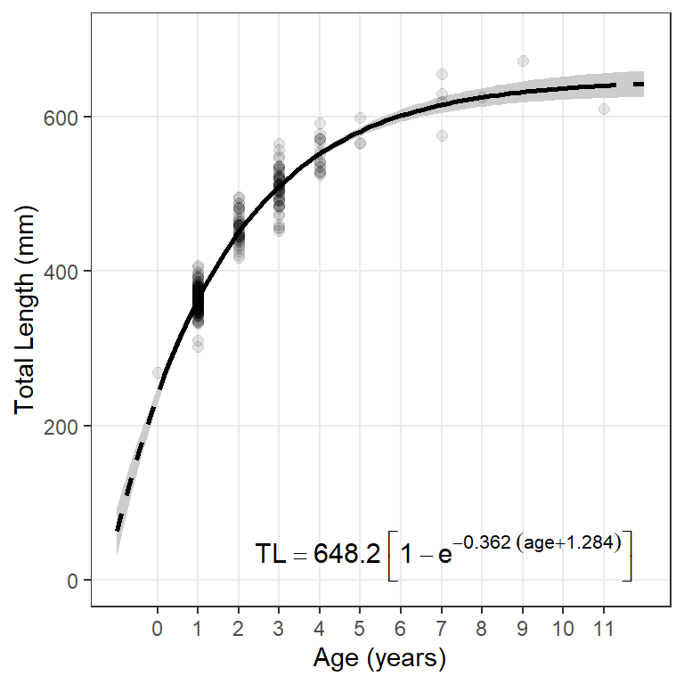
Warning
The large parentheses created by bgroup in the equation will not render properly under Windows using R v4.2.2. I posted about this on StackOverlow and was told that it was a Windows-only bug in v4.2.2. It has been fixed in v4.2.3 under which this post was rendered.
References
Ogle, D. H. 2016. Introductory Fisheries Analyses with R. CRC Press, Boca Raton, FL.
Ogle, D. H., T. O. Brenden, and J. L. McCormick. 2017. Growth Estimation: Growth Models and Statistical Inference. Pages 265–359 in M. C. Quist and D. A. Isermann, editors. Age and Growth of Fishes: Principles and Techniques. American Fisheries Society, Bethesda, MD.
Reuse
Citation
BibTeX citation:
@online{h._ogle2019,
  author = {H. Ogle, Derek},
  title = {Von {Bertalanffy} {Growth} {Plots} {I}},
  date = {2019-12-31},
  url = {https://fishr-core-team.github.io/fishR/blog/posts/2019-12-31_vonB_plots_1/},
  langid = {en}
}
For attribution, please cite this work as:
H. Ogle, D. 2019, December 31. von Bertalanffy Growth Plots I. https://fishr-core-team.github.io/fishR/blog/posts/2019-12-31_vonB_plots_1/.