Ridgeline Length Frequency Plots

Note

The following packages are loaded for use below. I also set the default ggplot theme to theme_bw() for a classic “black-and-white” plot (rather than the default plot with a gray background).

library(FSA)
library(dplyr)        # for filter(), mutate(), select()
library(ggplot2)
library(ggridges)     # for geom_density_ridges(), stat_density_ridges(), et al.
theme_set(theme_bw())

 

Lake Superior Kiyi

Wilke described ridgeline plots as “partially overlapping line plots that create the impression of a mountain range.” I would describe them as partially overlapping density plots (akin to a smoothed histogram).

I thought that ridgeline plots might provide a nice visualization of length frequencies over time. For example, Lepak et al. (2017) examined (among other things) the lengths of Kiyi (Coregonus kiyi) captured in trawl tows in Lake Superior from 2003 to 2014. The length frequency data used in that paper is shown below (and stored in the lf object). Figure 1 is a modified version¹ of the length frequency histograms we included in the paper.

¹ Stripped of code that increased fonts, changed colors, etc.

#R|       year mon  tl
#R|  1    2003 May 183
#R|  2    2003 May 259
#R|  3    2004 May 200
#R|  9149 2004 Jul  77
#R|  9150 2004 Jul  87
#R|  9151 2004 Jul  81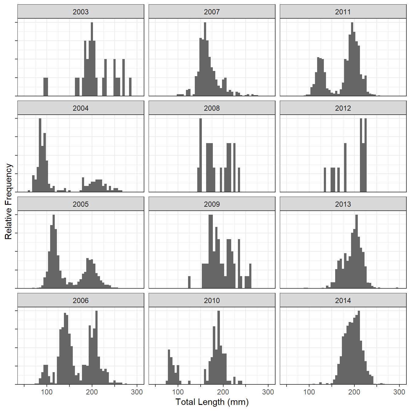

Figure 1: Histograms of the total lengths of Lake Superior Kiyi from 2003 to 2014.

 

Figure 2 is a near default joyplot of the same data.

ggplot(lf,aes(x=tl,y=year)) +
  geom_density_ridges() +
  scale_x_continuous(name="Total Length (mm)") +
  scale_y_discrete(expand=expansion(mult=c(0.01,0.16))) +
  theme(axis.title.y=element_blank())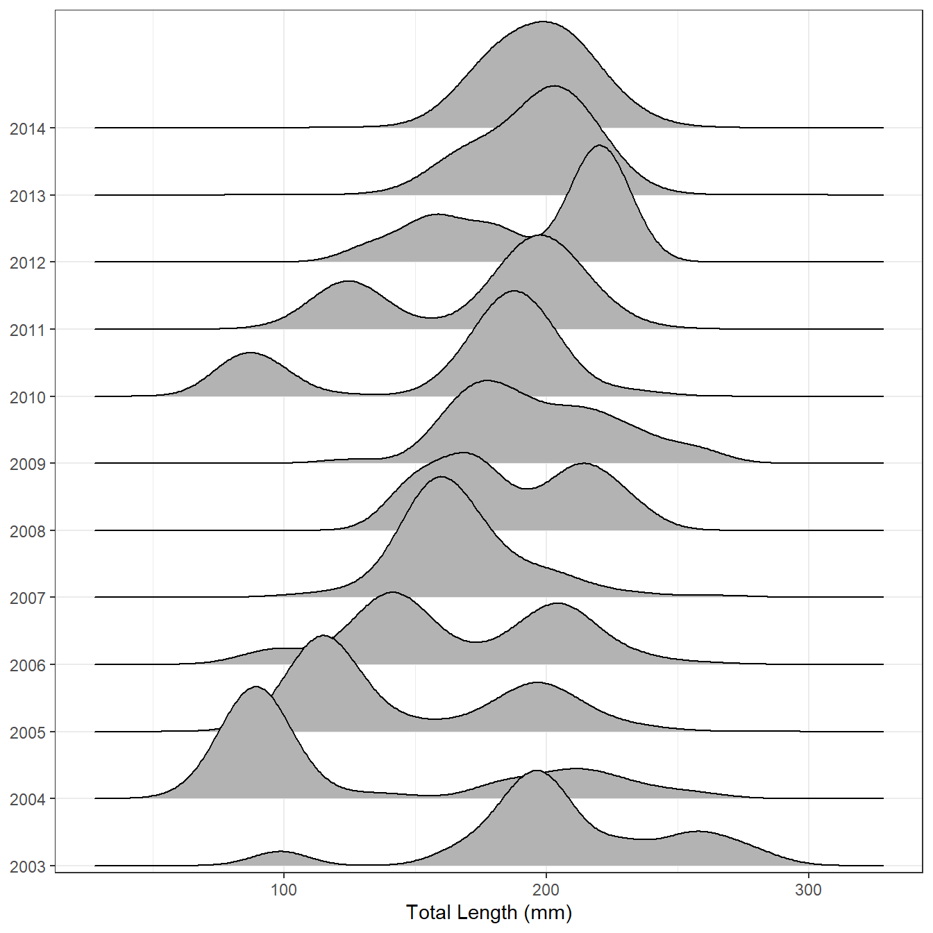

Figure 2: Ridgelinle plot of the total lengths of Lake Superior Kiyi from 2003 to 2014.

 

In my opinion, it is easier on the ridgeline plot to follow the strong year-classes that first appear in 2004 and 2010 through time and to see how fish in the strong year-classes grow and eventually merge in size with older fish. Thus, ridgeline plots look useful for displaying length (or age) data across many groups (years, locations, etc.).²

² Wilkeillustrates many possible modifications to the ridgeline plots including adding data points, show summary statistics, or using histograms rather than densities.

 

Lake Erie Walleye

The following code use the WalleyeErie2 data frame built-in to FSA. This provides an example with data that you can run on your own. I include some bells-and-whistles from Wilke’s demonstration.

# reduce data to one location and make sure year variable is a factor
data(WalleyeErie2,package="FSAdata")
we2 <- WalleyeErie2 |>
  filter(loc==2) |>
  mutate(fyear=as.factor(year))

ggplot(we2,aes(x=tl,y=fyear,fill=0.5-abs(0.5-after_stat(ecdf)))) +
  stat_density_ridges(geom="density_ridges_gradient",calc_ecdf=TRUE,scale=1) +
  scale_x_continuous(name="Total Length (mm)") +
  scale_y_discrete(expand=expansion(mult=c(0.01,0.05))) +
  scale_fill_viridis_c(name="Tail Probability",guide="none") +
  theme(axis.title.y=element_blank())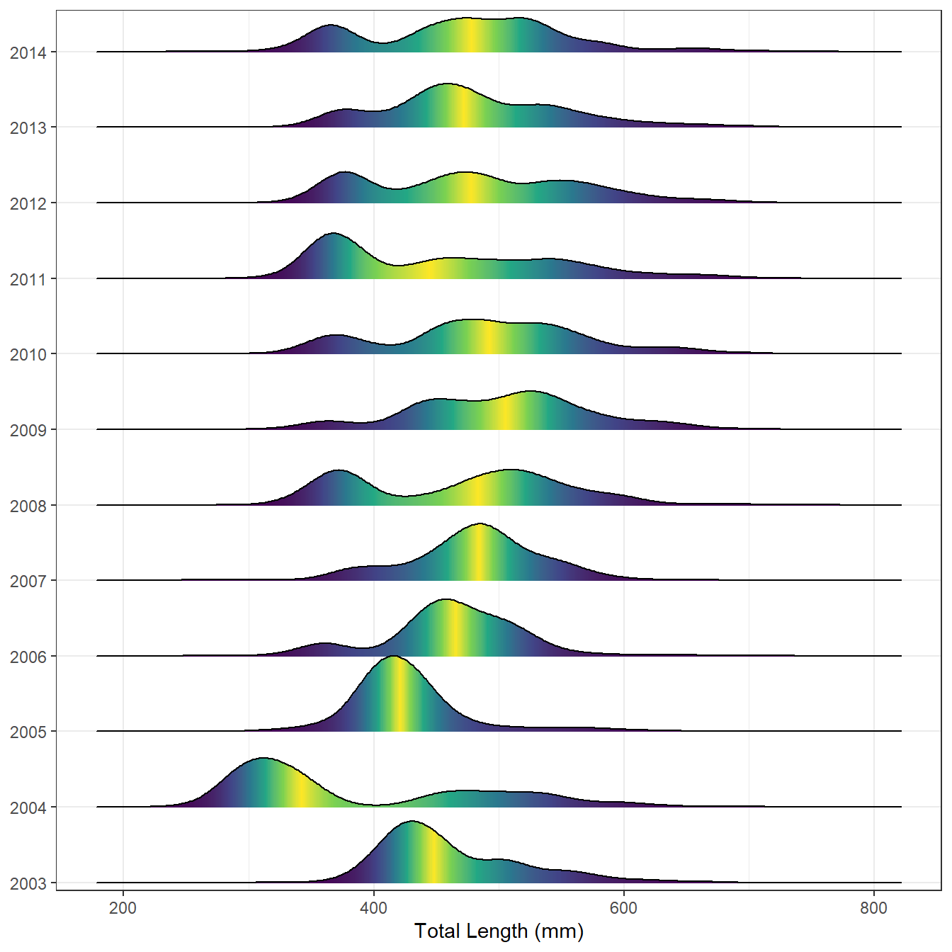

Figure 3: Ridgelinle plot of the total lengths of Lake Erie Walleye from 2003 to 2014.

References

Lepak, T. A., D. H. Ogle, and M. R. Vinson. 2017. Age, year-class strength variability, and partial age validation of Kiyis from Lake Superior. North American Journal of Fisheries Management 37:1151–1160.

Reuse

Citation

BibTeX citation:

@online{h. ogle2017,
  author = {H. Ogle, Derek},
  title = {Ridgeline {Length} {Frequency} {Plots}},
  date = {2017-07-28},
  url = {https://fishr-core-team.github.io/fishR//blog/posts/2017-7-28_LF_Ridgeline_Plot},
  langid = {en}
}

For attribution, please cite this work as:

H. Ogle, D. 2017, July 28. Ridgeline Length Frequency Plots. https://fishr-core-team.github.io/fishR//blog/posts/2017-7-28_LF_Ridgeline_Plot.