Deriving Starting Values for Growth Functions in FSA

Derek H. Ogle

2025-04-24

Introduction

The most common growth models used in fisheries, such as von Bertalanffy, Gompertz, logistic, and Richards, are non-linear models. Computer functions used to estimate parameters for these models require “starting values” to initiate the parameter search algorithm. Previous versions of FSA (v0.9.6 and lower) used ad hoc methods to estimate starting values for parameterizations of the von Bertalanffy function, but did not provide any method to derive starting values for the ohter common growth functions.

Several “self-starting” non-linear models are provided in R, with three of these found in base R and one in an add-on package that correspond to the common fisheries growth models. These functions provide starting values that are based on robust theory. Herein, I show how the starting values provided by these self-starting functions can be used to derive starting values for the common parameterizations of the common growth models used in fisheries. I will conclude by briefly demonstrating a new function in FSA that will provide the starting values demonstrated here.

Derivation of Starting Values

von Bertalanffy Length-at-Age

FSA provides a wide variety of von Bertalanffy parameterizations for modeling simple length-at-age data (Table 1).¹

Table 1: Parameterizations of the von Bertalanffy growth equation for length-at-age data available in FSA.

param	Equation
1	$E(L_t) = L_\infty\left(1-e^{-K(t-t_0)}\right)$
2	$E(L_t) = L_\infty - (L_\infty-L_0)~e^{-Kt}$
3	$E(L_t) = \frac{\omega}{K}\left(1-e^{-K(t-t_0)}\right)$
4	$E(L_t) = L_\infty - (L_\infty-L_0)~e^{-\frac{\omega}{L_\infty}t}$
5	$E(L_t) = L_\infty\left(1-e^{-log(2)\frac{t-t_0}{t_{50}-t_0}}\right)$
6	$E(L_t) = L_r + (L_\infty-L_r)~e^{-e^{-K(t-t_r)}}$
7	$E(L_t) = L_1+(L_3-L_1)\frac{1-e^{-K(t-t_1)}}{1-e^{-K(t_3-t_1)}}$
8	$E(L_t) = L_1+(L_3-L_1)\frac{1-r^{2\frac{t-t_1}{t_3-t_1}}}{1-r^2}$ where $r=\frac{L_3-L_2}{L_2-L_1}$

The response variable, $L$, is length and the explanatory variable, $t$ is age. Parameters in these growth functions are:

• $L_\infty$ = asymptotic mean length
• $K$ = exponential rate of approach to $L_\infty$
• $t_0$ = nuisance parameter that is the hypothetical time/age when mean length is 0
• $L_0$ = mean length at age-0 (i.e., hatching or birth)
• $\omega$ = growth rate near $t_0$
• $t_{50}$ = age when half of $L_\infty$ is reached
• $t_r$ = mean age at $L_r$ (sometimes this is a constant)
• $L_r$ = mean length at $t_r$ (sometimes this is a constant)
• $L_1$ = mean length at $t_1$ (generally a younger age)
• $L_2$ = mean length at $t_2$ (generally an intermediate age)
• $L_3$ = mean length at $t_3$ (generally a older age)

Constant values (i.e., set by the user) are:

• $t_r$ = mean age at $L_r$ (sometimes this is a parameter)
• $L_r$ = mean length at $t_r$ (sometimes this is a parameter)
• $t_1$ = a younger (generally) age
• $t_2$ = an age halfway between $t_1$ and $t_2$
• $t_3$ = an older (generally) age

SSasymp() is a self-starting function² to fit an “asymptotic regression” function to data. The parameterization for this function is³

$$Y = \text{Asym}+(\text{R0}-\text{Asym})~e^{-e^{\text{lrc}\times\text{input}}}$$

where $Y$ and $\text{input}$ are the response and explanatory variables, respectively, $\text{Asym}$ is a parameter for the horizontal (i.e., $Y$) asymptote, $\text{R0}$ is a parameter related to the value of $Y$ at $X=0$, and $lrc$ is a “parameter representing the natural logarithm of the rate constant.”

In growth (in length) modeling, $Y$ is $L$ (for length); $\text{input}$ is $t$ (for time as measured by age); $\text{Asym}$ is clearly $L_{\infty}$, the asympotic mean length; and $\text{R0}$ is clearly $L_0$, the mean length at $t=0$ (i.e., the y-intercept). Thus, at this point, the R “asymptotic regression” function can be re-written for the purposes of growth modeling as

$$L = L_\infty - (L_\infty-L_0)~e^{-e^{\text{lrc}\times t}}$$

If we move $\text{lrc}$ off of the log scale by defining $K=e^{\text{lrc}}$, we can further write this function as

$$L = L_\infty - (L_\infty-L_0)~e^{-Kt} \qquad(1)$$

Equation 1 is exactly the second parameterization of the von Bertalanffy growth function in FSA.⁴ Thus, the starting values produced by SSasymp() can be used directly to find starting values for the second parameterization of the von Bertalanffy growth function in FSA (Table 2). Indeed these values can be used for all parameterizations that have $L_\infty$, $L_0$, and $K$. Starting values for other parameters in other parameterizations are derived from these values as shown below.

A starting value for $t_0$, the “hypothetical time when the mean length is zero”, is derived by setting $L=0$ in Equation 1 and solving for $t$.

$$\begin{align} 0 &= L_\infty - (L_\infty-L_0)~e^{-Kt} \\ L_\infty &= (L_\infty-L_0)~e^{-Kt} \\ \frac{L_\infty}{L_\infty-L_0} &= e^{-Kt} \\ log\left(\frac{L_\infty}{L_\infty-L_0}\right) &= -K \\ -\frac{log\left(\frac{L_\infty}{L_\infty-L_0}\right)}{K} &= t \end{align}$$

The $\omega$ parameter was introduced into the fisheries growth modeling literature as $\omega=KL_\infty$ (Gallucci and Quin 1979⁵). Thus, a starting value for $\omega$ is simply the product of the starting values for $K$ and $L_\infty$.

A starting value for $t_{50}$ is derived (most easily) by solving the first parameterization equation for $t$ when $\frac{L}{L_\infty}=\frac{1}{2}$.

$$\begin{align} L &= L_\infty\left(1-e^{-K(t-t_0)}\right) \\ \frac{L}{L_\infty} &= 1-e^{-K(t-t_0)} \\ \frac{1}{2} &= 1-e^{-K(t_{50}-t_0)} \\ e^{-K(t_{50}-t_0)} &= \frac{1}{2} \\ -K(t_{50}-t_0) &= log\left(\frac{1}{2}\right) \\ t_{50}-t_0 &= \frac{log(2)}{K} \\ t_{50} &= t_0+\frac{log(2)}{K} \end{align}$$

A starting value for $L_r$ (i.e., mean length at time $t_r$) can be found by simply plugging $t_r$ into any parameterization⁶ and solving for $L$. This strategy generalizes to find starting values for $L_1$, $L_2$, and $L_3$.

A starting value for $t_r$ can be found by plugging $L_r$ for $L$ into any of the parameterizations and solving for $t$.

Table 2: Conversion from SSasymp() parameters ($\text{Asym}$, $\text{R0}$, and $\text{lrc}$) to parameters for the common von Bertalanffy parameterizations used to model fish growth in FSA. Note that parameterizations 6, 7, and 8 have other parameters not shown in this table (but described in the main text).

Param	$L_\infty$	$L_0$	$K$	$\omega$	$t_0$	$t_{50}$
1	$\text{Asym}$		$e^{\text{lrc}}$		$-\frac{log\left(\frac{L_\infty}{L_\infty-L_0}\right)}{K}$
2	$\text{Asym}$	$\text{R0}$	$e^{\text{lrc}}$
3			$e^{\text{lrc}}$	$KL_\infty$	$-\frac{log\left(\frac{L_\infty}{L_\infty-L_0}\right)}{K}$
4	$\text{Asym}$	$\text{R0}$		$KL_\infty$
5	$\text{Asym}$				$-\frac{log\left(\frac{L_\infty}{L_\infty-L_0}\right)}{K}$	$t_0+\frac{log(2)}{K}$
6	$\text{Asym}$		$e^{\text{lrc}}$
7			$e^{\text{lrc}}$

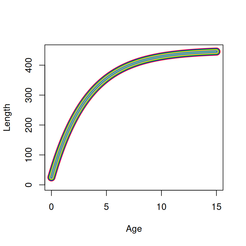
The equivalency of the parameterizations and the starting values across parameterizations is shown in Figure 1.

Figure 1: Parameterizations 1-8 of the von Bertalanffy growth functions evaluated at starting values derived from the parameters of SSasymp ($\text{Asym}$=450, $\text{R0}$=25, and $lrc$=-1.2). The linewidth decreases from the first to last parameterization (and the color differs) to show how the curves are plotted on top of each other.

The ninth parameterization (Table 3) of the von Bertalanffy model in FSA is a so-called “double von Bertalanffy” model.⁷

Table 3: Parameterizations of the von Bertalanffy growth equation for length-at-age data available in FSA.

param	Equation
9	$E(L_t) = L_\infty\frac{\left(1-e^{-K_2(t-t_0)}\right)\left(1+e^{-b(t-t_0-a)}\right)}{\left(1+e^{ab}\right)^{-\frac{K_2K_1}{b}}}$

Starting values for the ninth parameterization (i.e., the “double”) von Bertalanffy growth model have not been developed in FSA. Starting values for this parameterization will have to be developed by other means.

von Bertalanffy Seasonal Length-at-Age

There are also several parameterizations of the von Bertalanffy model that include a seasonal component in the model for when age is not recorded annually (Table 4).

Table 4: Parameterizations of the von Bertalanffy growth equation for length-at-age data with a seasonal component available in FSA.

param	Equation
10	$E(L_t) = L_\infty\left[1-e^{-K(t-t_0)-S(t)+S(t_0)}\right]$ where $S(t)=\frac{CK}{2\pi} sin(2\pi(t-t_s))$
11	$E(L_t) = L_\infty\left[1-e^{-K(t-t_0)-R(t)+R(t_0)}\right]$ where $R(t)=\frac{CK}{2\pi} sin(2\pi(t-WP+0.5))$
12	$E(L_t) = L_\infty(1-e^{-K'(t'-t_0)-V(t')+V(t_0)})$ where $V(t)= \frac{K'(1-NGT)}{2\pi}sin(\frac{2\pi}{(1-NGT)}(t-t_s))$

New parameters in these growth functions are:⁸

• $C$ = proportional growth depression at “winter peak”
• $t_s$ = time from $t=0$ until first growth oscillation begins
• $WP$ = “winter peak” (point of slowest growth)
• $K'$ = exponential rate of approach to $L_\infty$ during the growth period
• $NGT$ = length of “no-growth period”

Starting values for $L_\infty$, $K$, and $t_0$ are derived as if the data were recorded as annual lengths-at-age. Starting values for the other parameters are defined ad hoc as follows.

• $C$ set at an intermediate value of 0.5
• $t_s$ set at 0.3, a likely fraction of the year for growth to start in the northern hemisphere.
• $WP$ set at 0.8, because $WP=t_2+0.5$
• $NGT$ set at 0.3, a likely fraction of the year for “no growth” in the northern hemisphere.
• $K'$ set at $\frac{K}{(1-NGT)}$, assuming that $K$ was only over the “growth period” (i.e., $1-NGT$).

Starting values for the seasonal growth models are much less tested than those for annual growth models. Please consider them carefully.

von Bertalanffy Tag-Recapture

Still other parameterizations of the von Bertalanffy model are used with tag-recapture data (Table 5).

Table 5: Parameterizations of the von Bertalanffy growth equation for length at tag and recapture data available in FSA.

param	Equation
13	$E(L_r-L_m)=(L_\infty-L_m)\left(1-e^{-K\delta t}\right)$
14	$E(L_r)=L_m + (L_\infty-L_m)\left(1-e^{-K\delta t}\right)$
15	$E(L_r-L_m)=(L_\infty+\beta(L_m-\bar{L}_m)-L_m)\left(1-e^{-K\delta t}\right)$
16	$E(L_r-L_m)=(\alpha+\beta L_m)\left(1-e^{-K\delta t}\right)$
17	$E(L_r)=L_m+(\alpha+\beta L_m)\left(1-e^{-K\delta t}\right)$
18	$E(L_r-L_m)=\left[\frac{L_2g_1-L_1g_2}{g_1-g_2}-L_m\right]\left[1-\left(1+\frac{g_1-g_2}{L_1-L_2}\right)^{\delta t}\right]$
19	$E(L_r-L_m)=\left[\frac{L_2g_1-L_1g_2}{g_1-g_2}-L_m\right]\left[1-\left(1+\frac{g_1-g_2}{L_1+L_2}\right)^{t_2-t_1+S_2-S_1}\right]$ with $S_1=u\text{sin}\left(\frac{2\pi(t_1-w)}{2\pi}\right)$ and $S_2=u\text{sin}\left(\frac{2\pi(t_2-w)}{2\pi}\right)$

The response variable is generally the change in length (i.e., growth increment) from time of tagging to time of recapture, $L_r-L_m$. Some models are parameterized to have $L_m$ on the right-hand-side though. The explanatory variable is the change in time between the time of tagging and recapture, $\delta t$.

New parameters in these growth functions are:

• $\beta$ = a measure of individual fish variability.
• $\alpha$ = a nuisance parameter related to $L_\infty$ and an individual’s $L_m$.
• $g_1$ = mean annual growth rate at the (relatively small) reference length $L_1$.
• $g_2$ = mean annual growth rate at the (relatively large) reference length $L_2$.
• $u$ = describes “the extent of seasonality” ($u$=0 is no seasonality).
• $w$ = is the time of year when growth rates are maximum.

Starting values for (most of) these parameters were developed with the following ad hoc procedure.

• Regress (linear) observed annual growth rate (i.e., $\frac{\delta L}{\delta t}$ or $\frac{L_r-L_m}{t_r-t_m}$) on observed length-at-marking (i.e., $L_m$).
• Use this model to predict annual growth rates ($g_1$ and $g_2$) at $L_1$ and $L_2$. [$L_1$ and $L_2$ are chosen by the user in parameterization 18, but are set in FSA at the 10th and 90th percentiles of observed $L_m$ for the other parameterizations.]
• Use these results in $L_\infty=\frac{L_2g_1-L_1g_2}{L1-L2}$ and $K=-log\left[1+\frac{g_1-g_2}{L_1-L_2}\right]$ from Francis (1988).

In the Wang models $\beta$ is 0 if there is no individual variation in growth. In my experience a starting value for $\beta$ near 0, but no 0, is usually sufficient. FSA defaults to use $\beta=0.1$ as a starting value. A starting value for $\alpha$ of $L_\infty-\bar{L}_m$ is used by noting that if $\beta=0$ then parameterizations 15 and 16 are equal when $\alpha=L_\infty-L_m$. An average $\alpha$ can be estimated by using $\bar{L}_m$ for $L_m$. These starting values for $\alpha$ and $\beta$ have not been rigorously tested.

Warning

Starting values for parameterization 19 have not been developed for FSA. Starting values for this parameterization will have to be developed by other means.

Gompertz Length-at-Age

FSA provides several parameterizations of the Gompertz function for modeling simple length-at-age data (Table 6).

Table 6: Parameterizations of the Gompertz growth equation for length-at-age data available in FSA.

param	Equation
1	$E(L_t) = L_\infty e^{-e^{a_1-g_it}}$
2	$E(L_t) = L_\infty e^{-e^{-g_i(t-t_i)}}$
3	$E(L_t) = L_0 e^{a_2(1-e^{-g_it})}$
4	$E(L_t) = L_\infty e^{-a_2e^{-g_it}}$
5	$E(L_t) = L_\infty e^{-\frac{1}{g_i}e^{-g_i(t-t_0)}}$

New parameters in these growth functions are:⁹

• $t_i$ = age at the inflection point
• $g_i$ = instantaneous growth rate at $t_i$, the inflection point
• $a_1$, $a_2$ = nuisance parameters with no biological meaning

SSgompertz() is a self-starting function¹⁰ to fit a Gompertz function to data. The parameterization for this function is¹¹

$$Y = \text{Asym}~e^{-b_2b_3^X}$$

where $Y$ and $X$ are the response and explanatory variables, respectively, $\text{Asym}$ is a parameter for the horizontal (i.e., $Y$) asymptote, $b_2$ is a parameter related to the value of $Y$ at $X=0$, and $b_3$ is a “parameter related to the scale of the x-axis.”

In growth (in length) modeling, $Y$ is $L$ (for length), $X$ is $t$ (for time as measured by age), and $\text{Asym}$ is clearly $L_{\infty}$. Thus, at this point, the Gompertz function from SSgompertz() can be re-written for the purposes of growth modeling as

$$L = L_\infty e^{-b_2b_3^t} \qquad(2)$$

It is not immediately clear how $b_2$ and $b_3$ relate to parameters from common parameterizations of the Gompertz functions used to model fish growth. These will be explained below.

The first parameterization differs from Equation 2 only in the exponent of $e$ (after the negative). This part of the equation for the first parameterization can be rearranged as follows

$$\begin{align} & e^{(a-g_it)} \\ & e^{a_1}e^{-g_it)} \end{align}$$

If $b_2=e^{a_1}$ and $b_3=e^{-g_i}$ then this simplified exponent is the same as the exponent in Equation 2. Thus, $g_i=-log(b_3)$ and $a_1=log(b_2)$ (and, of course, $L_\infty=\text{Asym}$).

Similarly, the second parameterization also only differs from Equation 2 after the negative in the exponent of $e$. Again, simplifying this exponent gives

$$\begin{align} & e^{-g_i(t-t_i)} \\ & e^{-g_it+g_it_i} \\ & e^{-g_it}e^{g_it_i} \\ & e^{g_it_i}e^{-g_it} \end{align}$$

If $b_2=e^{g_it_i}$ and $b_3=e^{-g_i}$ then this simplified exponent is the same as the exponent in Equation 2. Thus, $g_i=-log(b_3)$ and $t_i=\frac{log(b_2)}{g_i}$.

There is no asymptote in the third parameterizations, so the entire function must be manipulated to show equivalence to Equation 2.

$$\begin{align} & L_0 e^{a_2(1-e^{-g_it})} \\ & L_0 e^{a_2-a_2e^{-g_it}} \\ & L_0 e^{a_2}e^{-a_2e^{-g_it}} \\ \end{align}$$ If $L_\infty=L_0e^{a_2}$, $b_2=a_{2}$, and, again, $b_3=e^{-g_i}$ then the third parameterization is equivalent to Equation 2. Thus, $a_2=b_2$, $g_i=-log(b_3)$, and $L_0=\frac{L_\infty}{e^{a_2}}$.

The fourth parameterization is equal to Equation 2 if $b_2=a_2$ and $b_3=e^{-g_i}$. Thus, again $a_2=b_2$ and $g_i=-log(b_3)$ (and, of course, $L_\infty=\text{Asym}$).

The fifth parameterization includes $t_0$ which appears to be defined, as in the von Bertalanffy function, as the age where the mean length is zero (i.e., the x-intercept). The three-parameter Gompertz function used here has a lower asymptote at $L=0$ and, thus, does not have an x-intercept. Therefore, it is not exactly clear what $t_0$ is. However, again, the exponent of $e$ (after the negative) of the fifth parameterizations can be rearranged

$$\begin{align} & \frac{1}{g_i}e^{-g_i(t-t_0)} \\ & \frac{1}{g_i}e^{-g_it+g_it_0} \\ & \frac{1}{g_i}e^{-g_it}e^{g_it_0} \\ & \frac{1}{g_i}e^{g_it_0}e^{-g_it} \end{align}$$

If $b_2=\frac{1}{g_i}e^{g_it_0}$ and $b_3=e^{-g_i}$, then this simplified exponent is the same as the exponent in Equation 2. Thus, $g_i=-log(b_3)$ and $t_0=\frac{log(b_2g_i)}{g_i}$ (and, of course, $L_\infty=\text{Asym}$).

These findings are summarized in Table 7.

Table 7: Conversion from SSgompertz() parameters ($\text{Asym}$, $b_2$, and $b_3$) to parameters for the common Gompertz parameterizations used to model fish growth in FSA.

param	$L_\infty$	$L_0$	$g_i$	$t_i$	$t_0$	$a_{\text{\#}}$
1	$\text{Asym}$		$-log(b_3)$			$log(b_2)$
2	$\text{Asym}$		$-log(b_3)$	$\frac{log(b_2)}{g_i}$
3		$\frac{L_\infty}{e^{b_2}}$	$-log(b_3)$			$b_2$
4	$\text{Asym}$		$-log(b_3)$			$b_2$
5	$\text{Asym}$		$-log(b_3)$		$\frac{log(b_2g_i)}{g_i}$

The equivalency of the parameterizations and the starting values across parameterizations is shown in Figure 2.

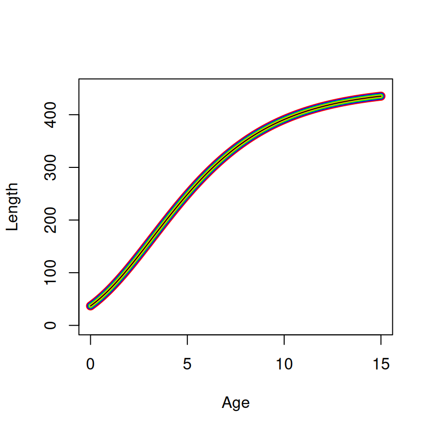
Figure 2: All parameterizations of the Gompertz growth functions evaluated at starting values derived from the parameters of SSgompertz ($\text{Asym}$=450, $b_2$=2.5, and $b_3$=0.75). The linewidth decreases from the first to last parameterization (and the color differs) to show how the curves are plotted on top of each other.

Gompertz Tag-Recapture

Still other parameterizations of the Gompertz model are used with tag-recapture data (Table 8).

Table 8: Parameterizations of the Gompertz growth equation for length at tag and recapture data available in FSA.

param	Equation
6	$E(L_r-L_m)=L_{\infty}\left[\frac{L_m}{L_{\infty}}\right]^{e^{-g_i\delta t}}-L_m$
7	$E(L_r)=L_{\infty}\left[\frac{L_m}{L_{\infty}}\right]^{e^{-g_i\delta t}}$

Warning

Starting values for the tag-recapture growth models have not been developed for FSA. Starting values for these parameterizations will have to be developed by other means.

Logistic Length-at-Age

FSA provides several parameterizations of the logistic function for modeling simple length-at-age data (Table 9).

Table 9: Parameterizations of the logistic growth equation for length-at-age data available in FSA.

param	Equation
1	$E(L_t) = \frac{L_\infty}{1+e^{-g_{-\infty}(t-t_i)}}$
2	$E(L_t) = \frac{L_\infty}{1+ae^{-g_{-\infty}t}}$
3	$E(L_t) = \frac{L_0L_\infty}{L_0+(L_\infty - L_0)e^{-g_{-\infty}t}}$

The response variable, $L$, is the mean length and the explanatory variable, $t$ is age. Parameters in these growth functions are:¹²

• $g_{-\infty}$ is the instantaneous growth rate at $t=-\infty$
• $a$ = nuisance parameters with no biological meaning

SSlogis() is a self-starting function¹³ to fit a logistic function to data. The parameterization for this function is¹⁴

$$Y = \frac{\text{Asym}}{1+e^{\frac{\text{xmid}-\text{input}}{\text{scal}}}}$$

where $Y$ and $\text{input}$ are the response and explanatory variables, respectively, $\text{Asym}$ is a parameter for the horizontal (i.e., $Y$) asymptote, $xmid$ is a parameter for the value of $X$ at the inflection point, and $scal$ is a “parameter on the input axis.”

In growth (in length) modeling, $Y$ is $L$ (for length), $\text{input}$ is $t$ (for time as measured by age), and $\text{Asym}$ is clearly $L_{\infty}$. Most likely $xmid$ is $t_i$, but it is not clear at this point. Thus, at this point, the R logistic function can be re-written for the purposes of growth modeling as

$$L = \frac{L_\infty}{1+e^{\frac{\text{xmid}-t}{\text{scal}}}} \qquad(3)$$

Below I show how parameters in the common parameterizations of the logistic function relate to $\text{xmid}$ and $\text{scal}$ (and, possibly, $L_{\infty}$). It is easier to relate Equation 3 to the Gompertz paramaeterizations if Equation 3 is presented in the more verbose form of

$$\begin{align} L &= \frac{L_\infty}{1+e^{\frac{\text{xmid}-t}{\text{scal}}}} \\ &= \frac{L_\infty}{1+e^{\frac{\text{xmid}}{\text{scal}}-\frac{t}{\text{scal}}}} \\ &= \frac{L_\infty}{1+e^{\frac{\text{xmid}}{\text{scal}}}e^{-\frac{t}{\text{scal}}}} \end{align} \qquad(4)$$

The only difference between the first parameterization and Equation 3 is in the denominator after the “1+”. This portion of the equation for the first parameterization can be rewritten as

$$\begin{align} & e^{-g_{-\infty}(t-t_i)} \\ & e^{-g_{-\infty}t+g_{-\infty}t_i} \\ & e^{-g_{-\infty}t}e^{g_{-\infty}t_i} \\ & e^{g_{-\infty}t_i}e^{-g_{-\infty}t} \end{align}$$

Comparing this to Equation 4 it is apparent that $g_{-\infty}=\frac{1}{\text{scal}}$ and $g_{-\infty}t_i=\frac{\text{xmid}}{\text{scal}}$. The latter can be simplified as

$$\begin{align} g_{-\infty}t_i &= \frac{\text{xmid}}{\text{scal}} \\ t_i &= \frac{\text{xmid}}{g_{-\infty}\text{scal}} \\ t_i &= \frac{\text{xmid}g_{-\infty}}{g_{-\infty}} \\ t_i &= \text{xmid} \end{align}$$

Thus, $\text{xmid}$ is the abcissa of the inflection point. Starting values for the first parameterization are thus $L_\infty=\text{Asym}$, $g_{-\infty}=\frac{1}{\text{scal}}$, and $t_i=\text{xmid}$.

The second paramaterization only differs from Equation 3 in the denominator after the “1+”, and no simplification is needed to notice that $g_{-\infty}=\frac{1}{\text{scal}}$ and $a=e^{\frac{\text{xmid}}{\text{scal}}}$.

The third parameterizations differs more substantively and requires more work. First, rewrite the whole equation by dividing both the numerator and denominator by $L_0$ to get

$$L = \frac{L_\infty}{1+\frac{L_\infty - L_0}{L_0}e^{-g_{-\infty}t}}$$

In this form the only difference from Equation 3 is again in the denominator after the “1+”. Again, by comparing this to Equation 4, it is apparent that $g_{-\infty}=\frac{1}{\text{scal}}$ and $\frac{L_\infty - L_0}{L_0}=e^{\frac{\text{xmid}}{\text{scal}}}$. This second value is solved for $L_0$ with

$$\begin{align} \frac{L_\infty - L_0}{L_0} &= e^{\frac{\text{xmid}}{\text{scal}}} \\ L_\infty - L_0 &= L_0e^{\frac{\text{xmid}}{\text{scal}}} \\ L_\infty &= L_0 + L_0e^{\frac{\text{xmid}}{\text{scal}}} \\ L_\infty &= L_0\left(1+e^{\frac{\text{xmid}}{\text{scal}}}\right) \\ \frac{L_\infty}{1+e^{\frac{\text{xmid}}{\text{scal}}}} &= L_0 \end{align}$$

These findings are summarized in Table 10.

Table 10: Conversion from SSlogis() parameters ($\text{Asym}$, $\text{xmid}$, and $\text{scal}$) to parameters for the common logistic parameterizations used to model fish growth in FSA.

param	$L_\infty$	$L_0$	$g_{-\infty}$	$t_i$	$a$
1	$\text{Asym}$		$\frac{1}{\text{scal}}$	$\text{xmid}$
2	$\text{Asym}$		$\frac{1}{\text{scal}}$		$e^{\frac{\text{xmid}}{\text{scal}}}$
3	$\text{Asym}$	$\frac{L_\infty}{1+e^{\frac{\text{xmid}}{\text{scal}}}}$	$\frac{1}{\text{scal}}$

The equivalency of the parameterizations and the starting values across parameterizations is shown in Figure 3.

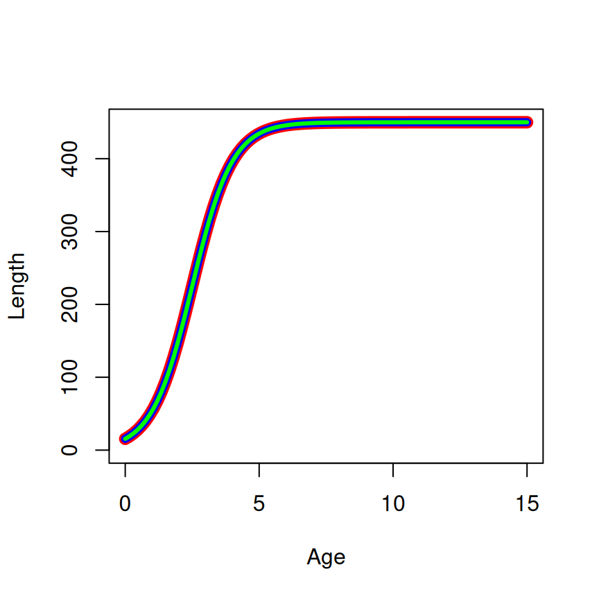
Figure 3: All parameterizations of the logistic growth functions evaluated at starting values derived from the parameters of SSlogis ($\text{Asym}$=450, $\text{xmid}$=2.5, and $\text{scal}$=0.75). The linewidth decreases from the first to last parameterization (and the color differs) to show how the curves are plotted on top of each other.

Richards Length-at-Age

FSA provides several parameterizations of the Richards function for modeling simple length-at-age data (Table 11).

Table 11: Parameterizations of the Richards growth equation for length-at-age data available in FSA.

param	Equation
1	$E(L_t) = L_\infty\left[1-\frac{1}{b}e^{-k(t-t_i)}\right]^{b}$
2	$E(L_t) = L_\infty\left(1+e^{-k(t-t_0)}\right)^{b}$
3	$E(L_t) = L_\infty\left[1+\left(\left(\frac{L_0}{L_\infty}\right)^{\frac{1}{b}}-1\right)e^{-kt}\right]^{b}$

The response variable, $L$, is the mean length and the explanatory variable, $t$ is age. New parameters in these growth functions are:¹⁵

• $k$ = growth rate parameter
• $b$ = nuisance parameter with no biological meaning

The FlexParamCurve package contains SSposnegRichards() which is a self-starting function for using nls() to fit a “Positive-Negative Richards growth” function to data. This function can fit an 8-parameter curve but if some of the parameters are not used then it is possible to fit a 4-parameter Richards function, a function similar to the Richards parameterizations in FSA. Their “twelfth model” (i.e., modno=12) can be written, using their R function parameters, as

$$Y = \frac{\text{Asym}}{\left[1+Me^{-K(X-\text{Infl})}\right]^{\frac{1}{M}}}$$ where $Y$ and $X$ are the response and explanatory variables, respectively, $\text{Asym}$ is a parameter for the horizontal (i.e., $Y$) asymptote, $K$ is a “rate parameter”, $\text{Infl}$ is the “inflection point” (i.e., the x-axis position of the inflection point), and $M$ is a “shape parameter”.

To better match the parameterizations in FSA, the FlexParamCurve function can be re-written as,

$$Y = \text{Asym}\left[1+Me^{-K(X-\text{Infl})}\right]^{-\frac{1}{M}}$$

In growth (in length) modeling, $Y$ is $L$ (for length), $X$ is $t$ (for time as measured by age). With these substitutions the (modified) function from FlexParamCurve can be re-written for the purposes of growth modeling as

$$L = L_\infty\left[1+Me^{-K(t-\text{Infl})}\right]^{-\frac{1}{M}} \qquad(5)$$

A comparison of Equation 5 to the three parameterizations of the Richards function in FSA clearly shows that $L_\infty=\text{Asym}$ and $b=-\frac{1}{M}$ for each. Substituting these values, and noting that $M=-\frac{1}{b}$, Equation 5 can be written as

$$L = L_\infty\left[1-\frac{1}{b}Me^{-K(t-\text{Infl})}\right]^{b}$$

This is exactly the first parameterization in FSA if $k=K$ and $t_i=\text{Infl}$. In fact, $k=K$ and $t_i=\text{Infl}$ in the other parameterizations.

If $t_0$ is the value of $t$ when $L=0$ then plug 0 into Equation 5 and solve for $t$ as follows¹⁶

$$\begin{align} 0 &= L_\infty\left[1+Me^{-K(t-\text{Infl})}\right]^{-\frac{1}{M}} \\ 0 &= 1+Me^{-K(t-\text{Infl})} \\ -\frac{1}{M} &= e^{-K(t-\text{Infl})} \\ log\left(-\frac{1}{M}\right) &= -K(t-\text{Infl}) \\ -\frac{log\left(-\frac{1}{M}\right)}{K} &= t-\text{Infl} \\ \text{Infl}-\frac{log\left(-\frac{1}{M}\right)}{K} &= t \end{align}$$ or, alternatively, $t_0=t_i-\frac{log(b)}{k}$.

In the third parameterization $L_0$ is defined as the mean length when $t=0$. Thus, plug $t=0$ into Equation 5 and solve for $L$ to see that $L_0=L_\infty\left[1-\frac{1}{b}e^{kt_i}\right]^{b}$.

These findings are summarized in Table 12.

Table 12: Conversion from SSposnegRichards() parameters ($\text{Asym}$, $\text{Infl}$, $K$, and $M$) to parameters for the common Richards parameterizations used to model fish growth in FSA.

param	$L_\infty$	$L_0$	$k$	$t_i$	$t_0$	$b$
1	$\text{Asym}$		$K$	$\text{Infl}$		$-\frac{1}{M}$
2	$\text{Asym}$		$K$		$\text{Infl}-\frac{log\left(\frac{1}{M}\right)}{K}$	$-\frac{1}{M}$
3	$\text{Asym}$	$\text{Asym}\left[1+Me^{K\times\text{Infl}}\right]^{-\frac{1}{M}}$	$K$			$-\frac{1}{M}$

The equivalency of the parameterizations and the starting values across parameterizations is shown in Figure 3.

Figure 4: All parameterizations of the Richards growth functions evaluated at starting values derived from the parameters of SSposnegrichards ($\text{Asym}$=450, $\text{Infl}$=2.5, $K$=0.5, $M$=0.1). The linewidth decreases from the first to last parameterization (and the color differs) to show how the curves are plotted on top of each other.

Schnute Length-at-Age

Schnute (1981) proposed a model for fish growth that can represent the von Bertalanffy, Gompertz, logistic, and Richards functions, along with others. The model has the following four parameters

• $L_1$ = expected length at (a relatively young) age $t_1$
• $L_3$ = expected length at (a relatively old) age $t_3$
• $a$ = a shape parameter that is inversely related to width of the “arc” before an inflection point
• $b$ = a shape parameter this is related to the ratio of the height of the “arcs” before and afer the inflection point

Starting values for $L_1$ and $L_3$ are easily obtained as the mean observed lengths at ages $t_1$ and $t_3$. However, I am unaware of any robust methodological method for developing starting values for $a$ and $b$. Descriptions in Schnute (1981) suggest that $a$ is equal to $K$ from the von Bertalanffy or $k$ from the Richards, if growth is shaped like those functions. A good “wild guess” at $K$ and $k$ is 0.3, so FSA used 0.3 as an ad hoc “wild guess” starting value for $a$. Further discussion in Schnute (1981) of the shape of growth trajectories relative to $a$ suggests that $a$ is likely not negative for most fisheries length-at-age data.

No similar observations were made with respect to $b$ from reading Schnute (1981). Limited personal experience suggests that using a starting value for $b$ are fickle. For cases 1 and 2, a “small” $b$ tends to work, so a starting value of 0.5 is used for $b$ in FSA. For case 3, a “larger” $b$ is needed, so a staring of 3.0 is used for $b$ in FSA. These starting values are “wild guess” at best and are unlikely to work in all (or even nost) situations. See the examples at the end of this article for how to manually choose starting values with FSA.

Finally, it seems that the automatic generation of stating values algorithm tends to work better if $t_1$ is very near, if not the actual, youngest observed age. In contrast, $t_3$ seems to work better if it is near the start (i.e., younger age) rather than the end of the asymptote.

Finding Starting Values in FSA

In FSA versions >0.9.6, findGrowthStarts() can be used to find the starting values described here. This function has four main parameters. The first two are a formula of the form length~age and data= which contain the length and age data from which the starting values will be derived. Additionally, use type= to choose the type of growth function to be used (i.e., "von Bertalanffy", "Gompertz", "logistic", or "Richards") and param= to choose the particularly parameterization for the model by the number shown in Table 1, Table 4, Table 6, Table 9, and Table 11.

For example, suppose that length-at-age data similar to that shown below is available in a data.frame named df.

#>  age tlV
#>    0  61
#>    2 237
#>    3 287
#>    4 312
#>    7 430
#>   15 435

The starting values for the first parameterization of the von Bertalanffy model could be obtained as below.

( sv1 <- findGrowthStarts(tlV~age,data=GrowthData1,type="von Bertalanffy",param=1) )
#>        Linf           K          t0 
#> 454.4806075   0.2974555  -0.4752262

It is also possible to declare the model parameterization with a “name.”¹⁷

( sv1 <- findGrowthStarts(tlV~age,data=GrowthData1,type="von Bertalanffy",pname="Typical") )
#>        Linf           K          t0 
#> 454.4806075   0.2974555  -0.4752262

There may be times when the provided starting values are non-sensical (you may get a warning message) or they do not lead to model convergence when fitting the non-linear regression to data. In these instances it may be useful to view a quick diagnostic plot of how the model evaluated at the starting values “fits” the data. Such a plot can be made by including plot=TRUE in findGrowthStarts().

sv1 <- findGrowthStarts(tlV~age,data=GrowthData1,type="von Bertalanffy",param=1,
                        plot=TRUE)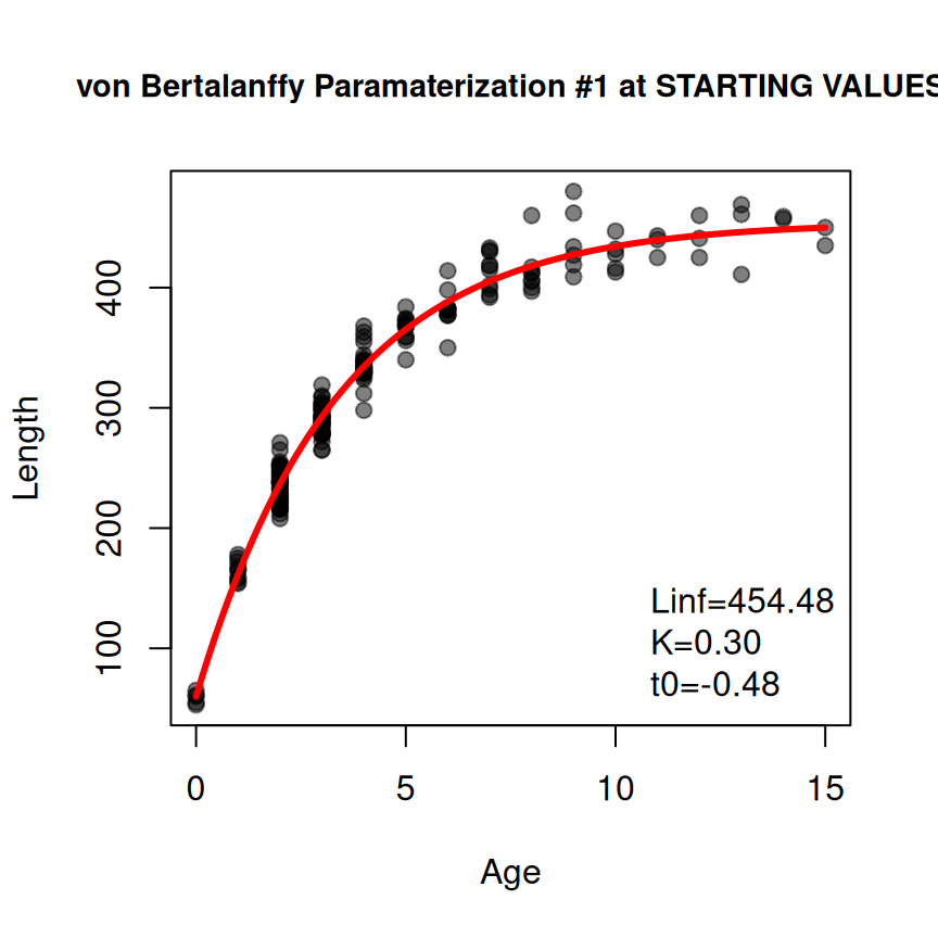

Additionally, it may be useful to “fix” some starting values at values of your choice (rather than having them determined from the data). Such parameters can be included in a NAMED vector given to fixed= in findGrowthStarts(). For example, the K parameter is fixed at 0.5 below.

( sv2 <- findGrowthStarts(tlV~age,data=GrowthData1,type="von Bertalanffy",param=1,
                          fixed=c("K"=0.5)) )
#>        Linf           K          t0 
#> 454.4806075   0.5000000  -0.2827173

Some parameterizations of the von Bertalanffy require the user to choose values for certain constants. For example, param=7 requires you to choose a “young” age for t1 and an “older” age for t2. These constants should be set in a NAMED vector that is given to constvals= in findGrowthStarts().

( sv3 <- findGrowthStarts(tlV~age,data=GrowthData1,type="von Bertalanffy",param=7,
                          constvals=c("t1"=1,"t3"=13)) )
#>          L1          L3           K 
#> 161.4312295 446.2251430   0.2974555

Of course, all of these optional arguments may be used together.¹⁸

sv4 <- findGrowthStarts(tlV~age,data=GrowthData1,type="von Bertalanffy",param=7,
                        constvals=c("t1"=1,"t3"=13),fixed=c("K"=0.5),plot=TRUE)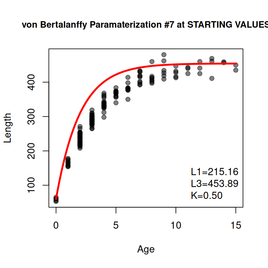

Of course, similar code is used for the other growth models (and parameterizations).

( sv5 <- findGrowthStarts(tlV~age,data=GrowthData1,type="Gompertz",param=2) )
#>        Linf          gi          ti 
#> 443.5949291   0.4521523   1.1615297

It is important to note that these are examples of find the starting values only. These starting values would then be provided to a nonlinear model fitting algorithm (e.g., nls()) to find the best-fit parameter estimates. This is demonstrated more thoroughly elsewhere, but below is a quick example using the starting values for first parameterization of von Bertalanffy derived above.

vonb1 <- makeGrowthFun(type="von Bertalanffy")
rvb1 <- nls(tlV~vonb1(age,Linf,K,t0),data=GrowthData1,start=sv1)
coef(rvb1)
#>        Linf           K          t0 
#> 456.0374952   0.2932701  -0.4848237