Creates a function for a specific parameterization of the von Bertalanffy and other common growth functions.
Source:R/makeGrowthFun.R
makeGrowthFun.RdCreates a function for a specific parameterizations of the von Bertalanffy, Gompertz, logistic, Richards, Schnute, and Schnute-Richards growth functions. The resulting function can be used to calculate length(s) from age(s) and specific growth function parameters, which is useful for model-fitting and plotting. Equations for each parameterization are shown in this article and with showGrowthFun.
Usage
makeGrowthFun(
  type = c("von Bertalanffy", "Gompertz", "logistic", "Richards", "Schnute",
    "Schnute-Richards"),
  param = 1,
  pname = NULL,
  case = NULL,
  simple = FALSE,
  msg = FALSE
)
Arguments
- type
A single string (i.e., one of “von Bertalanffy”, “Gompertz”, “logistic”, “Richards”, “Schnute”, “Schnute-Richards”) that indicates the type of growth function to show.
- param
A single numeric that indicates the specific parameterization of the growth function. Will be ignored if
pnameis non-NULL. See details.- pname
A single character that indicates the specific parameterization of the growth function. If
NULLthenparamwill be used. See details.- case
A numeric that indicates the specific case of the Schnute function to use.
- simple
A logical that indicates whether the function will accept all parameter values in the first parameter argument (
=FALSE; DEFAULT) or whether all individual parameters must be specified in separate arguments (=TRUE). See examples.- msg
A logical that indicates whether a message about the growth function and parameter definitions should be output (
=TRUE) or not (=FALSE; DEFAULT).
Value
Returns a function that can be used to predict fish size given a vector of ages and values for the growth function parameters and, in some parameterizations, values for constants. The result should be saved to an object that is then the function name. When the resulting function is used, the parameters are ordered as shown when the definitions of the parameters are printed after the function is called (if msg=TRUE). If simple=FALSE (DEFAULT), then the values for all parameters may be included as a vector in the first parameter argument (but in the same order). Similarly, the values for all constants may be included as a vector in the first constant argument (i.e., t1). If simple=TRUE, then all parameters and constants must be declared individually. The resulting function is somewhat easier to read when simple=TRUE, but is less general for some applications.
Details
Specific parameterizations can be chosen by including a name for the equation in `pname` or a number in `param=` (`param` will be ignored if `pname` is specificied). Specifics equations for the various parameterizations, along with parameter definitions, are in this article.
See this article and examples for how to use this function in the larger context of fitting growth models to data.
References
Ogle, D.H. 2016. Introductory Fisheries Analyses with R. Chapman & Hall/CRC, Boca Raton, FL.
Campana, S.E. and C.M. Jones. 1992. Analysis of otolith microstructure data. Pages 73-100 In D.K. Stevenson and S.E. Campana, editors. Otolith microstructure examination and analysis. Canadian Special Publication of Fisheries and Aquatic Sciences 117. [Was (is?) from https://waves-vagues.dfo-mpo.gc.ca/library-bibliotheque/141734.pdf.]
Fabens, A. 1965. Properties and fitting of the von Bertalanffy growth curve. Growth 29:265-289.
Francis, R.I.C.C. 1988. Are growth parameters estimated from tagging and age-length data comparable? Canadian Journal of Fisheries and Aquatic Sciences, 45:936-942.
Gallucci, V.F. and T.J. Quinn II. 1979. Reparameterizing, fitting, and testing a simple growth model. Transactions of the American Fisheries Society, 108:14-25.
Garcia-Berthou, E., G. Carmona-Catot, R. Merciai, and D.H. Ogle. A technical note on seasonal growth models. Reviews in Fish Biology and Fisheries 22:635-640.
Gompertz, B. 1825. On the nature of the function expressive of the law of human mortality, and on a new mode of determining the value of life contingencies. Philosophical Transactions of the Royal Society of London. 115:513-583.
Haddon, M., C. Mundy, and D. Tarbath. 2008. Using an inverse-logistic model to describe growth increments of blacklip abalone (Haliotis rubra) in Tasmania. Fishery Bulletin 106:58-71. [Was (is?) from https://spo.nmfs.noaa.gov/sites/default/files/pdf-content/2008/1061/haddon.pdf.]
Karkach, A. S. 2006. Trajectories and models of individual growth. Demographic Research 15:347-400. [Was (is?) from https://www.demographic-research.org/volumes/vol15/12/15-12.pdf.]
Katsanevakis, S. and C.D. Maravelias. 2008. Modeling fish growth: multi-model inference as a better alternative to a priori using von Bertalanffy equation. Fish and Fisheries 9:178-187.
Mooij, W.M., J.M. Van Rooij, and S. Wijnhoven. 1999. Analysis and comparison of fish growth from small samples of length-at-age data: Detection of sexual dimorphism in Eurasian perch as an example. Transactions of the American Fisheries Society 128:483-490.
Polacheck, T., J.P. Eveson, and G.M. Laslett. 2004. Increase in growth rates of southern bluefin tuna (Thunnus maccoyii) over four decades: 1960 to 2000. Canadian Journal of Fisheries and Aquatic Sciences, 61:307-322.
Quinn, T. J. and R. B. Deriso. 1999. Quantitative Fish Dynamics. Oxford University Press, New York, New York. 542 pages.
Quist, M.C., M.A. Pegg, and D.R. DeVries. 2012. Age and growth. Chapter 15 in A.V. Zale, D.L Parrish, and T.M. Sutton, editors. Fisheries Techniques, Third Edition. American Fisheries Society, Bethesda, MD.
Richards, F. J. 1959. A flexible growth function for empirical use. Journal of Experimental Biology 10:290-300.
Ricker, W.E. 1975. Computation and interpretation of biological statistics of fish populations. Technical Report Bulletin 191, Bulletin of the Fisheries Research Board of Canada. [Was (is?) from https://publications.gc.ca/collections/collection_2015/mpo-dfo/Fs94-191-eng.pdf.]
Ricker, W.E. 1979. Growth rates and models. Pages 677-743 In W.S. Hoar, D.J. Randall, and J.R. Brett, editors. Fish Physiology, Vol. 8: Bioenergetics and Growth. Academic Press, New York, NY. [Was (is?) from https://books.google.com/books?id=CB1qu2VbKwQC&pg=PA705&lpg=PA705&dq=Gompertz+fish&source=bl&ots=y34lhFP4IU&sig=EM_DGEQMPGIn_DlgTcGIi_wbItE&hl=en&sa=X&ei=QmM4VZK6EpDAgwTt24CABw&ved=0CE8Q6AEwBw#v=onepage&q=Gompertz%20fish&f=false.]
Schnute, J. 1981. A versatile growth model with statistically stable parameters. Canadian Journal of Fisheries and Aquatic Sciences, 38:1128-1140.
Schnute, J.T. and L.J. Richards. 1990. A unified approach to the analysis of fish growth, maturity, and survivorship data. Canadian Journal of Fisheries and Aquatic Sciences 47:24-40.
Somers, I. F. 1988. On a seasonally oscillating growth function. Fishbyte 6(1):8-11. [Was (is?) from https://www.fishbase.us/manual/English/fishbaseSeasonal_Growth.htm.]
Tjorve, E. and K. M. C. Tjorve. 2010. A unified approach to the Richards-model family for use in growth analyses: Why we need only two model forms. Journal of Theoretical Biology 267:417-425. [Was (is?) from https://www.researchgate.net/profile/Even_Tjorve/publication/46218377_A_unified_approach_to_the_Richards-model_family_for_use_in_growth_analyses_why_we_need_only_two_model_forms/links/54ba83b80cf29e0cb04bd24e.pdf.]
Tjorve, K. M. C. and E. Tjorve. 2017. The use of Gompertz models in growth analyses, and new Gompertz-model approach: An addition to the Unified-Richards family. PLOS One. [Was (is?) from https://doi.org/10.1371/journal.pone.0178691.]
Troynikov, V. S., R. W. Day, and A. M. Leorke. Estimation of seasonal growth parameters using a stochastic Gompertz model for tagging data. Journal of Shellfish Research 17:833-838. [Was (is?) from https://www.researchgate.net/profile/Robert_Day2/publication/249340562_Estimation_of_seasonal_growth_parameters_using_a_stochastic_gompertz_model_for_tagging_data/links/54200fa30cf203f155c2a08a.pdf.]
Vaughan, D. S. and T. E. Helser. 1990. Status of the Red Drum stock of the Atlantic coast: Stock assessment report for 1989. NOAA Technical Memorandum NMFS-SEFC-263, 117 p. [Was (is?) from https://repository.library.noaa.gov/view/noaa/5927/noaa_5927_DS1.pdf.]
Wang, Y.-G. 1998. An improved Fabens method for estimation of growth parameters in the von Bertalanffy model with individual asymptotes. Canadian Journal of Fisheries and Aquatic Sciences 55:397-400.
Weisberg, S., G.R. Spangler, and L. S. Richmond. 2010. Mixed effects models for fish growth. Canadian Journal of Fisheries And Aquatic Sciences 67:269-277.
Winsor, C.P. 1932. The Gompertz curve as a growth curve. Proceedings of the National Academy of Sciences. 18:1-8. [Was (is?) from https://pmc.ncbi.nlm.nih.gov/articles/PMC1076153/pdf/pnas01729-0009.pdf.]
See also
showGrowthFun to create an expression of the equation and findGrowthStarts to develop starting values for a growth function using the same type and pname/param arguments.
Author
Derek H. Ogle, DerekOgle51@gmail.com, thanks to Gabor Grothendieck for a hint about using get().
Examples
#===== Create typical von B function, calc length at single then multiple ages
vb <- makeGrowthFun()
vb(t=1,Linf=450,K=0.3,t0=-0.5)
#> [1] 163.0673
vb(t=1:5,Linf=450,K=0.3,t0=-0.5)
#> [1] 163.0673 237.4351 292.5280 333.3419 363.5775
#===== All parameters can be given to first parameter (default), unless simple=TRUE
vb(t=1,Linf=c(450,0.3,-0.5))
#> [1] 163.0673
vbS <- makeGrowthFun(simple=TRUE)
if (FALSE) vbS(t=1,Linf=c(450,0.3,-0.5)) # will error, parms must be separate # \dontrun{}
vbS(t=1,Linf=450,K=0.3,t0=-0.5)
#> [1] 163.0673
#===== Create original von B, first using param, then using pname
vbO <- makeGrowthFun(param=2)
vbO2 <- makeGrowthFun(pname="Original")
vbO(t=1:5,Linf=450,K=0.3,L0=25)
#> [1] 135.1523 216.7551 277.2079 321.9925 355.1697
vbO2(t=1:5,Linf=450,K=0.3,L0=25)
#> [1] 135.1523 216.7551 277.2079 321.9925 355.1697
#===== Create the third parameterization of the logistic growth function
# and show some details, and demo calculations
logi <- makeGrowthFun(type="logistic",param=3,msg=TRUE)
#> You have chosen paramaterization 3 (Karkach) of the logistic growth function.
#>
#> E[L|t] = L0*Linf/(L0+(Linf-L0)*exp(-gninf*t))
#>
#> where Linf = asymptotic mean length
#> gninif = instantaneous growth rate at t=-infinity
#> L0 = mean length at time/age 0
#>
logi(t=1:10,Linf=450,gninf=0.3,L0=25)
#> [1] 33.10306 43.56329 56.87790 73.52579 93.88275 118.10772 146.02049
#> [8] 177.01167 210.03562 243.72012
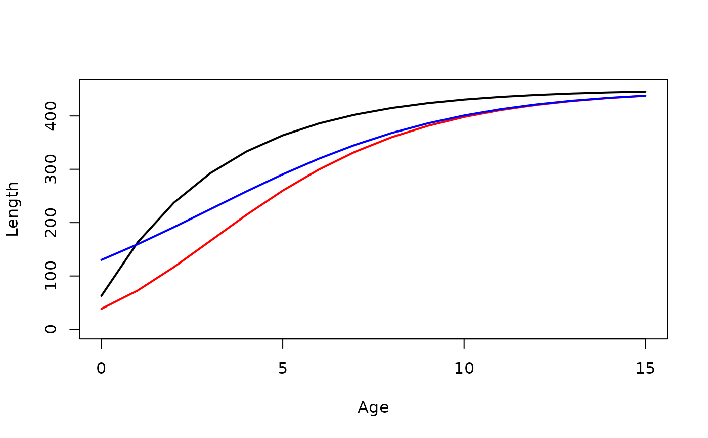
#===== Simple example of comparing several models
vb <- makeGrowthFun(type="von Bertalanffy")
gomp <- makeGrowthFun(type="Gompertz",param=2)
logi <- makeGrowthFun(type="logistic")
ages <- 0:15
vb1 <- vb(ages,Linf=450,K=0.3,t0=-0.5)
gomp1 <- gomp(ages,Linf=450,gi=0.3,ti=3)
logi1 <- logi(ages,Linf=450,gninf=0.3,ti=3)
plot(vb1~ages,type="l",lwd=2,ylim=c(0,450),ylab="Length",xlab="Age")
lines(gomp1~ages,lwd=2,col="red")
lines(logi1~ages,lwd=2,col="blue")
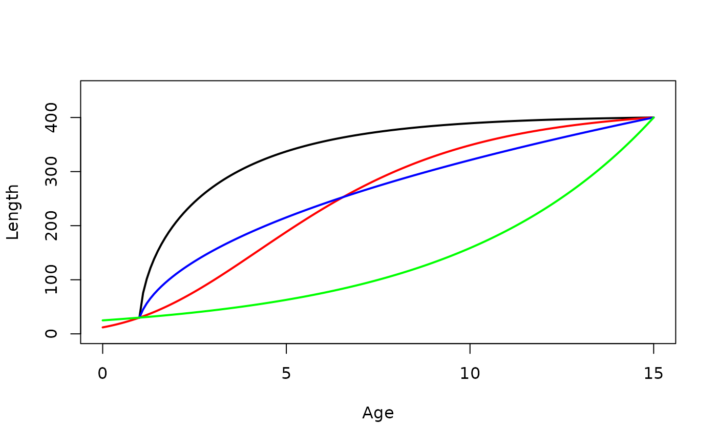
 #===== Simple example of four cases of Schnute model (note a,b choices)
Schnute1 <- makeGrowthFun(type="Schnute",case=1)
Schnute2 <- makeGrowthFun(type="Schnute",case=2)
Schnute3 <- makeGrowthFun(type="Schnute",case=3)
Schnute4 <- makeGrowthFun(type="Schnute",case=4)
ages <- seq(0,15,0.1)
s1 <- Schnute1(ages,L1=30,L3=400,a=0.3,b=2,t1=1,t3=15)
s2 <- Schnute2(ages,L1=30,L3=400,a=0.3, t1=1,t3=15)
s3 <- Schnute3(ages,L1=30,L3=400, b=2,t1=1,t3=15)
s4 <- Schnute4(ages,L1=30,L3=400, t1=1,t3=15)
plot(s1~ages,type="l",lwd=2,ylim=c(0,450),ylab="Length",xlab="Age")
lines(s2~ages,lwd=2,col="red")
lines(s3~ages,lwd=2,col="blue")
lines(s4~ages,lwd=2,col="green")
#===== Simple example of four cases of Schnute model (note a,b choices)
Schnute1 <- makeGrowthFun(type="Schnute",case=1)
Schnute2 <- makeGrowthFun(type="Schnute",case=2)
Schnute3 <- makeGrowthFun(type="Schnute",case=3)
Schnute4 <- makeGrowthFun(type="Schnute",case=4)
ages <- seq(0,15,0.1)
s1 <- Schnute1(ages,L1=30,L3=400,a=0.3,b=2,t1=1,t3=15)
s2 <- Schnute2(ages,L1=30,L3=400,a=0.3, t1=1,t3=15)
s3 <- Schnute3(ages,L1=30,L3=400, b=2,t1=1,t3=15)
s4 <- Schnute4(ages,L1=30,L3=400, t1=1,t3=15)
plot(s1~ages,type="l",lwd=2,ylim=c(0,450),ylab="Length",xlab="Age")
lines(s2~ages,lwd=2,col="red")
lines(s3~ages,lwd=2,col="blue")
lines(s4~ages,lwd=2,col="green")
 #===== Fitting the 8th parameterization of the von B growth model to data
# make von B function
vb8 <- makeGrowthFun(type="von Bertalanffy",param=8,msg=TRUE)
#> You have chosen paramaterization 8 (Francis) of the von Bertalanffy growth function.
#>
#> E[L|t] = L1+(L3-L1)*[(1-r^(2*[(t-t1)/(t3-t1)]))/(1-r^2)]
#>
#> where r = [(L3-L2)/(L2-L1)] and
#>
#> L1 = mean length at first (small) reference age
#> L2 = mean length at intermediate reference age
#> L3 = mean length at third (large) reference age
#>
#> You must also give values (i.e., they are NOT model parameters) for
#> t1 = first (usually a younger) reference age
#> t3 = third (usually an older) reference age
#>
# get starting values
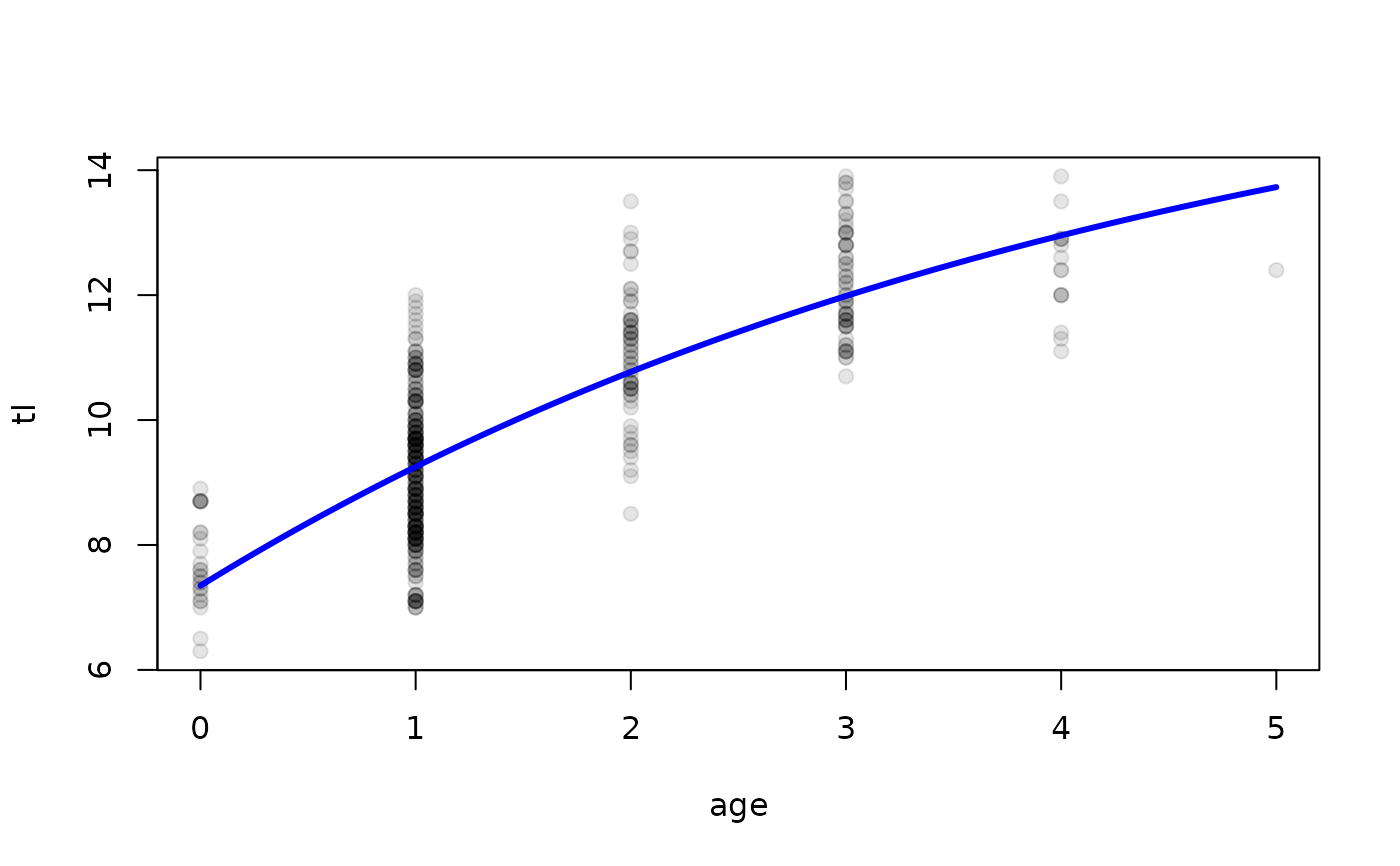
sv8 <- findGrowthStarts(tl~age,data=SpotVA1,type="von Bertalanffy",param=8,
constvals=c(t1=1,t3=5))
# fit function
nls8 <- nls(tl~vb8(age,L1,L2,L3,t1=c(t1=1,t3=5)),data=SpotVA1,start=sv8)
cbind(Est=coef(nls8),confint(nls8))
#> Waiting for profiling to be done...
#> Est 2.5% 97.5%
#> L1 9.251581 9.133607 9.369831
#> L2 11.985613 11.790010 12.181026
#> L3 13.729145 13.181939 14.349657
plot(tl~age,data=SpotVA1,pch=19,col=col2rgbt("black",0.1))
curve(vb8(x,L1=coef(nls8),t1=c(t1=1,t3=5)),col="blue",lwd=3,add=TRUE)
#===== Fitting the 8th parameterization of the von B growth model to data
# make von B function
vb8 <- makeGrowthFun(type="von Bertalanffy",param=8,msg=TRUE)
#> You have chosen paramaterization 8 (Francis) of the von Bertalanffy growth function.
#>
#> E[L|t] = L1+(L3-L1)*[(1-r^(2*[(t-t1)/(t3-t1)]))/(1-r^2)]
#>
#> where r = [(L3-L2)/(L2-L1)] and
#>
#> L1 = mean length at first (small) reference age
#> L2 = mean length at intermediate reference age
#> L3 = mean length at third (large) reference age
#>
#> You must also give values (i.e., they are NOT model parameters) for
#> t1 = first (usually a younger) reference age
#> t3 = third (usually an older) reference age
#>
# get starting values
sv8 <- findGrowthStarts(tl~age,data=SpotVA1,type="von Bertalanffy",param=8,
constvals=c(t1=1,t3=5))
# fit function
nls8 <- nls(tl~vb8(age,L1,L2,L3,t1=c(t1=1,t3=5)),data=SpotVA1,start=sv8)
cbind(Est=coef(nls8),confint(nls8))
#> Waiting for profiling to be done...
#> Est 2.5% 97.5%
#> L1 9.251581 9.133607 9.369831
#> L2 11.985613 11.790010 12.181026
#> L3 13.729145 13.181939 14.349657
plot(tl~age,data=SpotVA1,pch=19,col=col2rgbt("black",0.1))
curve(vb8(x,L1=coef(nls8),t1=c(t1=1,t3=5)),col="blue",lwd=3,add=TRUE)