Visualize Points Selected on a Calcified Structure
Derek H. Ogle
2023-12-19
Source:vignettes/seeRadiiData.Rmd
seeRadiiData.RmdIntroduction
A method for visualizing annular points that a user (or users)
selected on a calcified structure is described in this vignette. This
vignette assumes that you have an R data file or files created from
selecting points on a calcified structure using
digitizeRadii() as described in the Collecting Radial Measurements
vignette. It also assumes that you understand the language and functions
introducted in that vignette.
This vignette will use the following R data files:
- “Scale_1_DHO.rds”: annular points selected on the “Scale_1.jpg” file in the Collecting Radial Measurements vignette.
- “Scale_1_ODH.rds”: a second set of annular points selected on the “Scale_1.jpg” file in the Collecting Radial Measurements vignette.
- “Scale_1_OHD.rds”: a third set of annular points selected on the “Scale_1.jpg” file in the Collecting Radial Measurements vignette.
- “Oto140306_DHO.rds”: annular points selected on the “Oto140306.jpg” file. In contrast to the previous images, this image had a 1-mm scale-bar. This R data file was created with the following code.
digitizeRadii("Oto140306.jpg",id="140306",reading="DHO",
              description="Used to demonstrate use of scale-bar.",
              scaleBar=TRUE,scaleBarLength=1,edgeIsAnnulus=TRUE,
              windowSize=12)
Only the RFishBC package is needed for this
vignette.
Visualize One Set of Annuli
You can review the selected annuli on a structure with
showDigitizedImage(), which requires only the name of an R
data file created from digitizeRadii().1
showDigitizedImage("Scale_1_DHO.rds")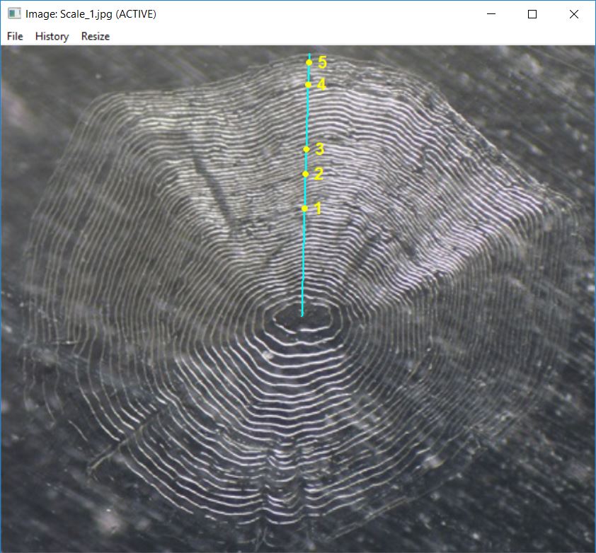
The plotting character, color, and relative size of the selected
points may be changed with pch.show=,
col.show=, and cex.show=, respectively. By
default, the points are connected which will display as a linear
transect if makeTransect=TRUE (the default) was used when
selecting annuli in digitizeRadii(). The color and width of
the connected lines may be changed with col.connect= and
lwd.connect=. The connected lines may be excluded
altogether with connect=FALSE. Annuli will be numbered if
showAnnuliLabels=TRUE (the default) with label colors and
relative size changed with col.ann= and
cex.ann=, respectively. Annuli for which numbers are
plotted may be controlled with annuliLabels= (e.g., only
the first six plus several others after that are shown for the Kiyi
otolith below). Defaults for all of these arguments may be set with
RFBCoptions() as was demonstrated in the Setting Arguments section of
this vignette
showDigitizedImage("Oto140306_DHO.rds",pch.show="+",col.show="blue",
                   col.connect="white",col.ann="black",cex.ann=1,
                   annuliLabels=c(1:6,8,10,13))
You can also just show the points without the transect and individually control the color of the annuli labels.
showDigitizedImage("Oto140306_DHO.rds",annuliLabels=c(1:6,8,10,13),
                   connect=FALSE,col.ann=c(rep("black",8),"white"),cex.ann=1)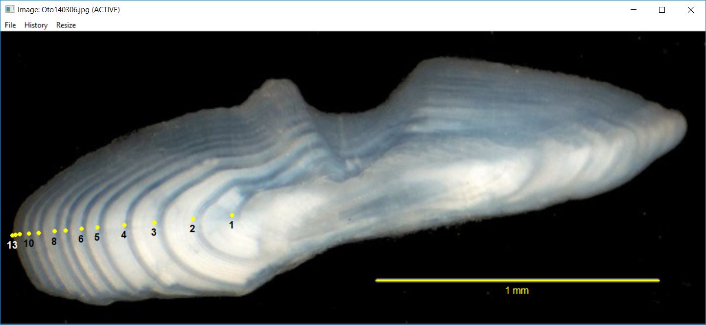
Visualize Multiple Readings of Same Structure
In some instances, you may be interested in visually comparing the
selected points from multiple readings of the same structure. The
showDigitizedImage() function can accomplish this if it is
given a vector of R data file names created from the same structure.
The listFiles() function (described in the Collecting Radial Measurements
vignette) may be used to identify all filenames in the current working
directory that have the file extension given in the first argument. For
example, all files with the “rds” extension are found below.
listFiles("rds")
#> [1] "DWS_Oto_89765_DHO.rds"  "Oto140306_DHO.rds"      "Oto140306_OHD.rds"
#> [4] "Scale_1_DHO.rds"        "Scale_1_ODH.rds"        "Scale_1_OHD.rds"
#> [7] "Scale_2_DHO.rds"        "Scale_2_OLDwNoNote.rds" "Scale_3_DHO.rds"
This list of names can be further filtered by including other key
words for the filenames in other=. For example, all files
with the “rds” extension that contain the keyword “Scale_1” are returned
below. For our purposes here, these filenames are saved into an object
(e.g., fns).
( fns <- listFiles("rds",other="Scale_1") )
#> [1] "Scale_1_DHO.rds" "Scale_1_ODH.rds" "Scale_1_OHD.rds"
The multiple readings of “Scale_1” can be seen by giving this set of
filenames to showDigitizedImage().2
showDigitizedImage(fns)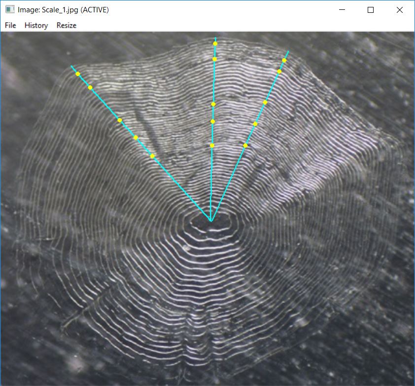
Aspects of the connecting lines and points may be controlled with
arguments to showDigitizedData(). For example, the code
below uses different colors for each set of connecting lines and
points.
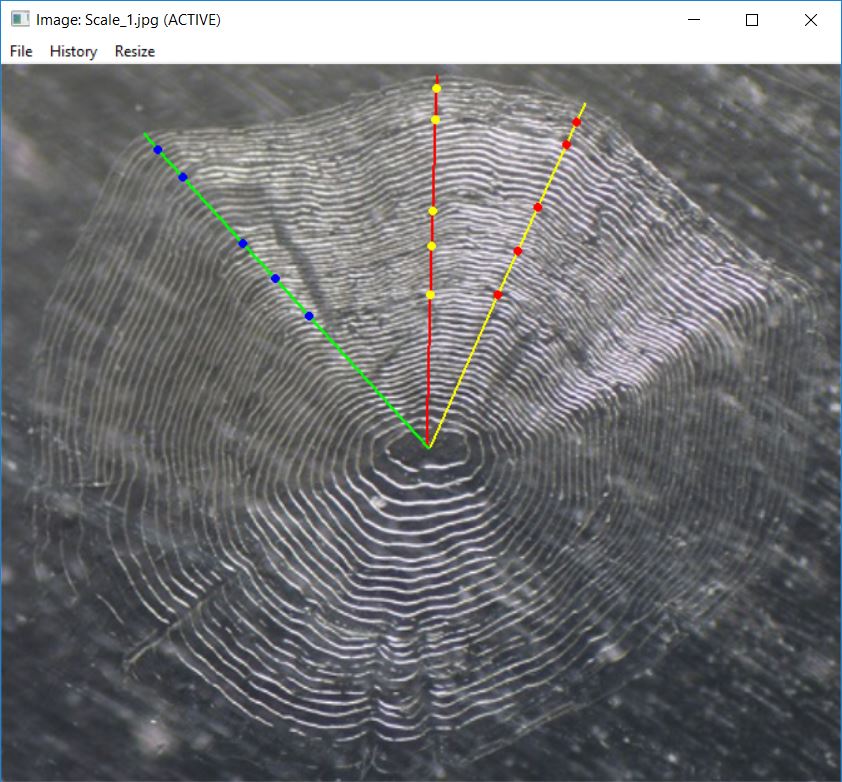
showDigitizedImage(fns,col.show=c("yellow","red","blue"),
                   col.connect=c("red","yellow","green"),lwd.connect=2)