Constructs plots of predicted weights at given lengths among different groups.

Constructs plots of predicted weights at given lengths among different groups. These plots allow the user to explore differences in predicted weights at a variety of lengths when the weight-length relationship is not the same across a variety of groups.

Usage

lwCompPreds(
  object,
  lens = NULL,
  qlens = c(0.05, 0.25, 0.5, 0.75, 0.95),
  qlens.dec = 1,
  base = exp(1),
  interval = c("confidence", "prediction", "both"),
  center.value = 0,
  lwd = 1,
  connect.preds = TRUE,
  show.preds = FALSE,
  col.connect = "gray70",
  ylim = NULL,
  main.pre = "Length==",
  cex.main = 0.8,
  xlab = "Groups",
  ylab = "Predicted Weight",
  yaxs = "r",
  rows = round(sqrt(num)),
  cols = ceiling(sqrt(num))
)

Arguments

object: An lm object (i.e., returned from fitting a model with lm). This model should have log(weight) as the response and log(length) as the explanatory covariate and an explanatory factor variable that describes the different groups.
lens: A numeric vector that indicates the lengths at which the weights should be predicted.
qlens: A numeric vector that indicates the quantiles of lengths at which weights should be predicted. This is ignored if lens is non-null.
qlens.dec: A single numeric that identifies the decimal place that the lengths derived from qlens should be rounded to (Default is 1).
base: A single positive numeric value that indicates the base of the logarithm used in the lm object in object. The default is exp(1), or the value e.
interval: A single string that indicates whether to plot confidence (="confidence"), prediction (="prediction"), or both (="both") intervals.
center.value: A single numeric value that indicates the log length used if the log length data was centered when constructing object.
lwd: A single numeric that indicates the line width to be used for the confidence and prediction interval lines (if not interval="both") and the prediction connections line. If interval="both" then the width of the prediction interval will be one less than this value so that the CI and PI appear different.
connect.preds: A logical that indicates whether the predicted values should be connected with a line across groups or not.
show.preds: A logical that indicates whether the predicted values should be plotted with a point for each group or not.
col.connect: A color to use for the line that connects the predicted values (if connect.preds=TRUE).
ylim: A numeric vector of length two that indicates the limits of the y-axis to be used for each plot. If null then limits will be chosen for each graph individually.
main.pre: A character string to be used as a prefix for the main title. See details.
cex.main: A numeric value for the character expansion of the main title. See details.
xlab: A single string for labeling the x-axis.
ylab: A single string for labeling the y-axis.
yaxs: A single string that indicates how the y-axis is formed. See par for more details.
rows: A single numeric that contains the number of rows to use on the graphic.
cols: A single numeric that contains the number of columns to use on the graphic.

Value

None. However, a plot is produced.

IFAR Chapter

7-Weight-Length.

References

Ogle, D.H. 2016. Introductory Fisheries Analyses with R. Chapman & Hall/CRC, Boca Raton, FL.

Author

Derek H. Ogle, DerekOgle51@gmail.com

Examples

# add log length and weight data to ChinookArg data
ChinookArg$logtl <- log(ChinookArg$tl)
ChinookArg$logwt <- log(ChinookArg$w)
# fit model to assess equality of slopes
lm1 <- lm(logwt~logtl*loc,data=ChinookArg)
anova(lm1)
#> Analysis of Variance Table
#> 
#> Response: logwt
#>            Df Sum Sq Mean Sq  F value    Pr(>F)    
#> logtl       1 92.083  92.083 898.4819 < 2.2e-16 ***
#> loc         2  2.634   1.317  12.8526 1.005e-05 ***
#> logtl:loc   2  0.101   0.051   0.4932     0.612    
#> Residuals 106 10.864   0.102                       
#> ---
#> Signif. codes:  0 ‘***’ 0.001 ‘**’ 0.01 ‘*’ 0.05 ‘.’ 0.1 ‘ ’ 1

# set graphing parameters so that the plots will look decent
op <- par(mar=c(3.5,3.5,1,1),mgp=c(1.8,0.4,0),tcl=-0.2)
# show predicted weights (w/ CI) at the default quantile lengths
lwCompPreds(lm1,xlab="Location")

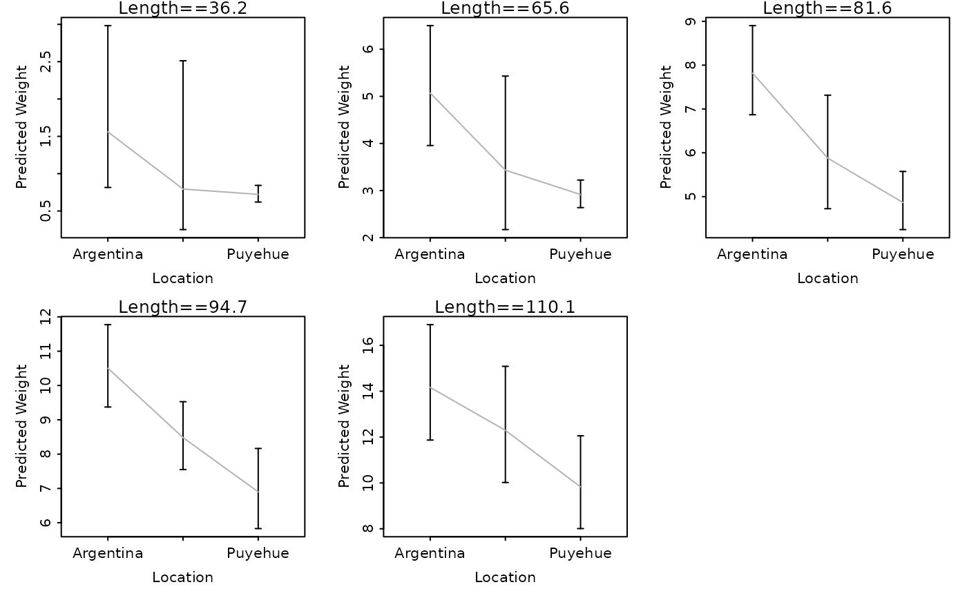
# show predicted weights (w/ CI) at the quartile lengths
lwCompPreds(lm1,xlab="Location",qlens=c(0.25,0.5,0.75))

# show predicted weights (w/ CI) at certain lengths
lwCompPreds(lm1,xlab="Location",lens=c(60,90,120,150))

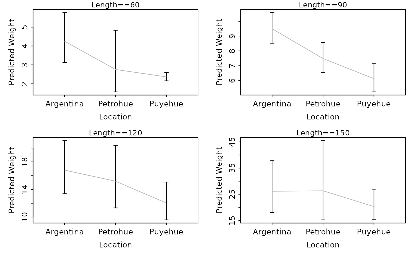
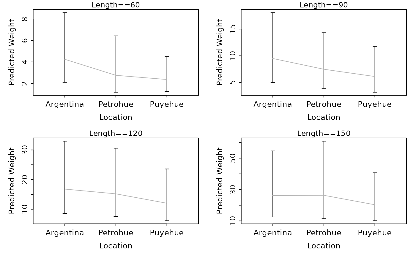
# show predicted weights (w/ just PI) at certain lengths
lwCompPreds(lm1,xlab="Location",lens=c(60,90,120,150),interval="prediction")

lwCompPreds(lm1,xlab="Location",lens=c(60,90,120,150),connect.preds=FALSE,show.preds=TRUE)


# fit model with a different base (plot should be the same as the first example)
ChinookArg$logtl <- log10(ChinookArg$tl)
ChinookArg$logwt <- log10(ChinookArg$w)
lm1 <- lm(logwt~logtl*loc,data=ChinookArg)
lwCompPreds(lm1,base=10,xlab="Location")

## return graphing parameters to original state
par(op)