Computes the Leslie or DeLury population estimate from catch and effort data.

Computes the Leslie or DeLury estimates of population size and catchability coefficient from paired catch and effort data. The Ricker modification may also be used.

Usage

depletion(
  catch,
  effort,
  method = c("Leslie", "DeLury", "Delury"),
  Ricker.mod = FALSE
)

# S3 method for depletion
summary(object, parm = c("all", "both", "No", "q", "lm"), verbose = FALSE, ...)

# S3 method for depletion
coef(object, parm = c("all", "both", "No", "q", "lm"), ...)

# S3 method for depletion
confint(
  object,
  parm = c("all", "both", "No", "q", "lm"),
  level = conf.level,
  conf.level = 0.95,
  ...
)

# S3 method for depletion
anova(object, ...)

# S3 method for depletion
rSquared(object, digits = getOption("digits"), percent = FALSE, ...)

# S3 method for depletion
plot(
  x,
  xlab = NULL,
  ylab = NULL,
  pch = 19,
  col.pt = "black",
  col.mdl = "gray70",
  lwd = 1,
  lty = 1,
  pos.est = "topright",
  cex.est = 0.95,
  ...
)

Arguments

catch: A numeric vector of catches of fish at each time.
effort: A numeric vector of efforts expended at each time.
method: A single string that indicates which depletion method to use
Ricker.mod: A single logical that indicates whether to use the modification proposed by Ricker (=TRUE) or not (=FALSE, default).
object: An object saved from the removal call (i.e., of class depletion).
parm: A specification of which parameters are to be given confidence intervals, either a vector of numbers or a vector of names. If missing, all parameters are considered.
verbose: A logical that indicates whether a reminder of the method used should be printed with the summary results.
...: Additional arguments for methods.
level: Same as conf.level but used for compatibility with generic confint function.
conf.level: A single number that represents the level of confidence to use for constructing confidence intervals.
digits: The number of digits to round the rSquared result to.
percent: A logical that indicates if the rSquared result should be returned as a percentage (=TRUE) or as a proportion (=FALSE; default).
x: An object saved from the depletion call (i.e., of class depletion).
xlab: A label for the x-axis.
ylab: A label for the y-axis.
pch: A numeric that indicates the type of plotting character.
col.pt: A string that indicates the color of the plotted points.
col.mdl: A string that indicates the color of the fitted line.
lwd: A numeric that indicates the line width of the fitted line.
lty: A numeric that indicates the type of line used for the fitted line.
pos.est: A single string to identify where to place the estimated population estimate and catchability on the plot. Can be set to one of "bottomright", "bottom", "bottomleft", "left", "topleft", "top", "topright", "right" or "center" for positioning the estimated mortality rates on the plot. Typically "bottomleft" (DEFAULT) and "topright" will be “out-of-the-way” placements. Set pos.est to NULL to remove the estimated population size and catchability coefficient from the plot.
cex.est: A single numeric that identifies the character expansion value for the estimated population estimate and catchability placed on the plot.

Value

A list with the following items:

method A string that indicates whether the "Leslie" or "DeLury" model was used.
catch The original vector of catches.
effort The original vector of efforts.
cpe A computed vector of catch-per-unit-effort for each time.
KorE A computed vector of cumulative catch (K; Leslie method) or effort (E; DeLury method).
lm The lm object from the fit of CPE on K (Leslie method) or log(CPE) on E (DeLury method).
est A 2x2 matrix that contains the estimates and standard errors for No and q.

Details

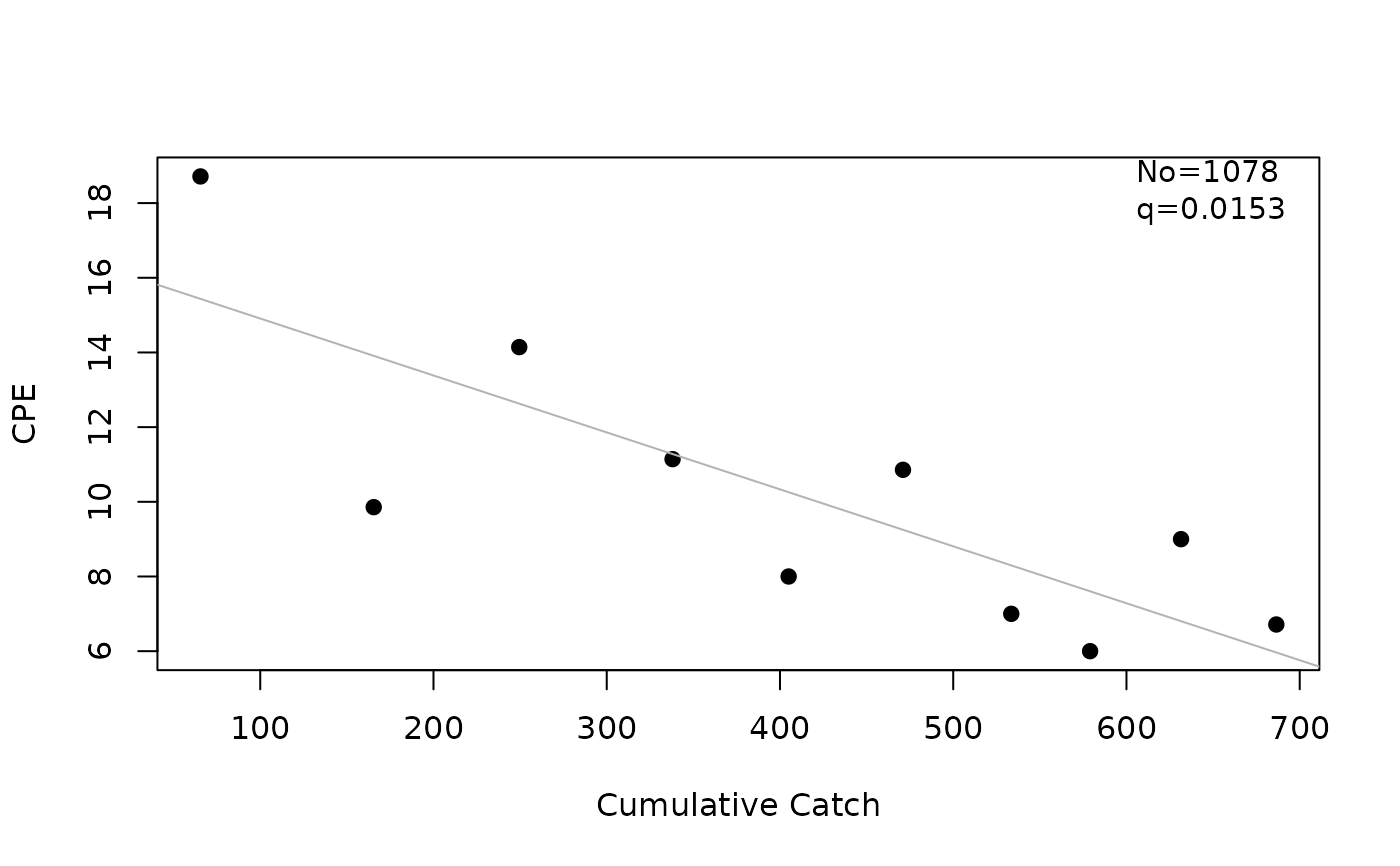
For the Leslie method, a linear regression model of catch-per-unit-effort on cumulative catch prior to the sample is fit. The catchability coefficient (q) is estimated from the negative of the slope and the initial population size (No) is estimated by dividing the intercept by the catchability coefficient. If Ricker.mod=TRUE then the cumulative catch is modified to be the cumulative catch prior to the sample plus half of the catch of the current sample.

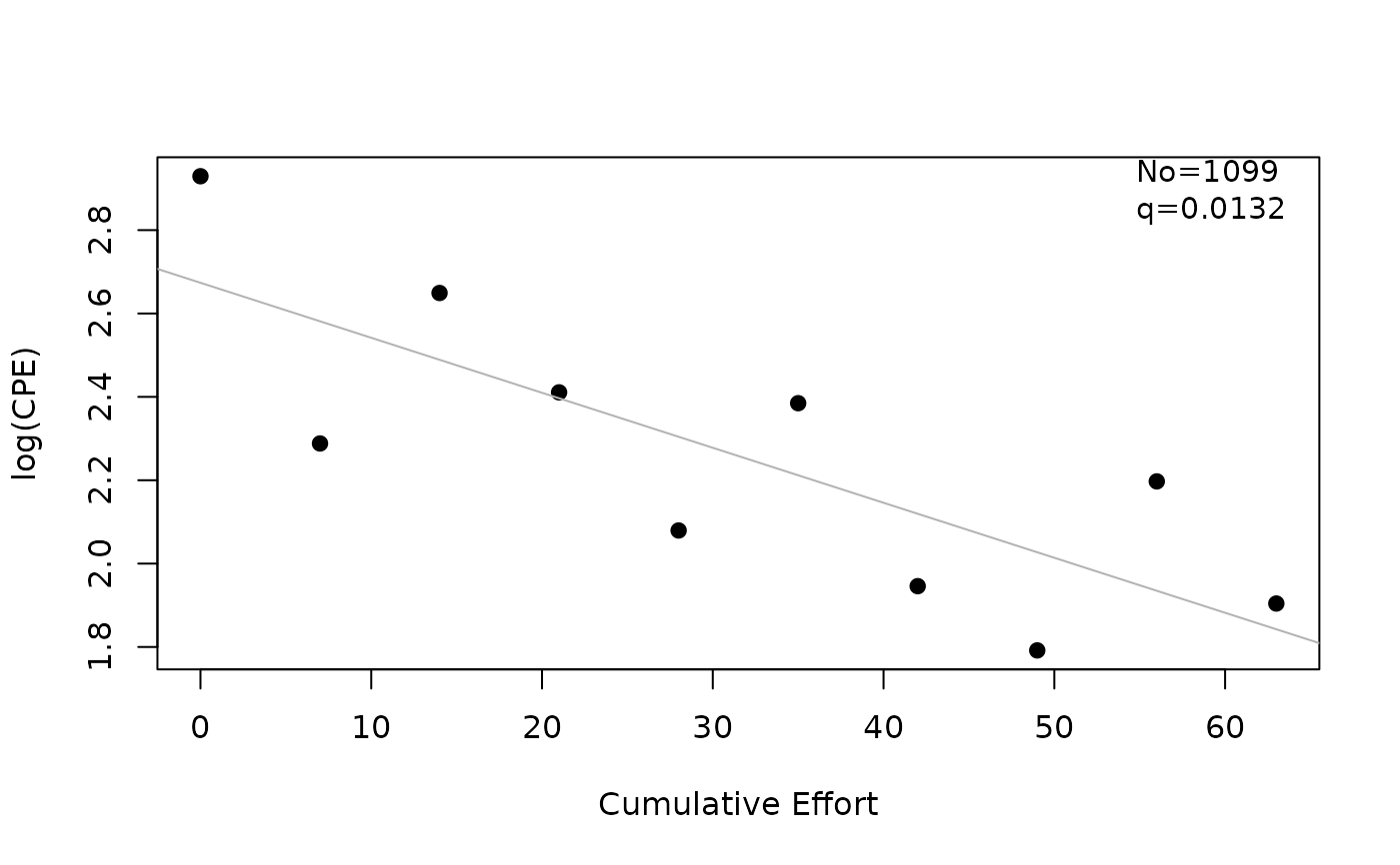
For the DeLury method, a linear regression model of log (catch-per-unit-effort) on cumulative effort is fit. The catchability coefficient (q) is estimated from the negative of the slope and the initial population size (No) is estimated by dividing the intercept as an exponent of e by the catchability coefficient. If Ricker.mod=TRUE then the cumulative effort is modified to be the cumulative effort prior to the sample plus half of the effort of the current sample.

Standard errors for the catchability and population size estimates are computed from formulas on page 298 (for Leslie) and 303 (for DeLury) from Seber (2002). Confidence intervals are computed using standard large-sample normal distribution theory with the regression error df.

testing

The Leslie method without the Ricker modification and the DeLury method with the Ricker modification matches the results from deplet in fishmethods for the darter (from fishmethods), LobsterPEI and BlueCrab from FSAdata, and SMBassLS for N0 to whole numbers, the SE for No to one decimal, q to seven decimals, and the SE of q to at least five decimals.

The Leslie method matches the results of Seber (2002) for N0, q, and the CI for Q but not the CI for N (which was so far off that it might be that Seber's result is incorrect) for the lobster data and the q and CI for q but the NO or its CI (likely due to lots of rounding in Seber 2002) for the Blue Crab data.

The Leslie and DeLury methods match the results of Ricker (1975) for No and Q but not for the CI of No (Ricker used a very different method to compute CIs).

IFAR Chapter

10-Abundance from Depletion Data.

References

Ogle, D.H. 2016. Introductory Fisheries Analyses with R. Chapman & Hall/CRC, Boca Raton, FL.

Ricker, W.E. 1975. Computation and interpretation of biological statistics of fish populations. Technical Report Bulletin 191, Bulletin of the Fisheries Research Board of Canada. [Was (is?) from http://www.dfo-mpo.gc.ca/Library/1485.pdf.]

Seber, G.A.F. 2002. The Estimation of Animal Abundance. Edward Arnold, Second edition (reprinted).

Author

Derek H. Ogle, DerekOgle51@gmail.com

Examples

## Leslie model examples
# no Ricker modification
l1 <- depletion(SMBassLS$catch,SMBassLS$effort,method="Leslie")
summary(l1)
#>        Estimate    Std. Err.
#> No 1.060296e+03 1.692676e+02
#> q  1.484403e-02 3.520491e-03
summary(l1,verbose=TRUE)
#> The Leslie method was used.
#>        Estimate    Std. Err.
#> No 1.060296e+03 1.692676e+02
#> q  1.484403e-02 3.520491e-03
summary(l1,parm="No")
#>    Estimate Std. Err.
#> No 1060.296  169.2676
rSquared(l1)
#> [1] 0.6896648
rSquared(l1,digits=1,percent=TRUE)
#> [1] 69
cbind(Est=coef(l1),confint(l1))
#>             Est      95% LCI      95% UCI
#> No 1.060296e+03 6.699638e+02 1.450627e+03
#> q  1.484403e-02 6.725759e-03 2.296229e-02
cbind(Est=coef(l1,parm="No"),confint(l1,parm="No"))
#>         Est  95% LCI  95% UCI
#> No 1060.296 669.9638 1450.627
cbind(Est=coef(l1,parm="q"),confint(l1,parm="q"))
#>          Est     95% LCI    95% UCI
#> q 0.01484403 0.006725759 0.02296229
summary(l1,parm="lm")
#> 
#> Call:
#> stats::lm(formula = cpe ~ K)
#> 
#> Residuals:
#>     Min      1Q  Median      3Q     Max 
#> -3.9373 -1.3879  0.3295  1.5023  2.9752 
#> 
#> Coefficients:
#>             Estimate Std. Error t value Pr(>|t|)    
#> (Intercept) 15.73906    1.51266  10.405 6.31e-06 ***
#> K           -0.01484    0.00352  -4.216  0.00293 ** 
#> ---
#> Signif. codes:  0 ‘***’ 0.001 ‘**’ 0.01 ‘*’ 0.05 ‘.’ 0.1 ‘ ’ 1
#> 
#> Residual standard error: 2.295 on 8 degrees of freedom
#> Multiple R-squared:  0.6897,	Adjusted R-squared:  0.6509 
#> F-statistic: 17.78 on 1 and 8 DF,  p-value: 0.00293
#> 
plot(l1)


# with Ricker modification
l2 <- depletion(SMBassLS$catch,SMBassLS$effort,method="Leslie",Ricker.mod=TRUE)
summary(l2)
#>        Estimate    Std. Err.
#> No 1.077571e+03 1.778035e+02
#> q  1.525078e-02 3.911632e-03
cbind(Est=coef(l2),confint(l1))
#>             Est      95% LCI      95% UCI
#> No 1.077571e+03 6.699638e+02 1.450627e+03
#> q  1.525078e-02 6.725759e-03 2.296229e-02
plot(l2)


## DeLury model examples
# no Ricker modification
d1 <- depletion(SMBassLS$catch,SMBassLS$effort,method="DeLury")
summary(d1)
#>        Estimate    Std. Err.
#> No 1.098503e+03 1.916049e+02
#> q  1.319375e-02 3.585777e-03
summary(d1,parm="q")
#>     Estimate   Std. Err.
#> q 0.01319375 0.003585777
summary(d1,verbose=TRUE)
#> The DeLury method was used.
#>        Estimate    Std. Err.
#> No 1.098503e+03 1.916049e+02
#> q  1.319375e-02 3.585777e-03
rSquared(d1)
#> [1] 0.6285719
cbind(Est=coef(d1),confint(d1))
#>             Est      95% LCI      95% UCI
#> No 1.098503e+03 6.566616e+02 1.540345e+03
#> q  1.319375e-02 4.924937e-03 2.146257e-02
summary(d1,parm="lm")
#> 
#> Call:
#> stats::lm(formula = log(cpe) ~ E)
#> 
#> Residuals:
#>      Min       1Q   Median       3Q      Max 
#> -0.29314 -0.21203  0.03796  0.16974  0.26238 
#> 
#> Coefficients:
#>              Estimate Std. Error t value Pr(>|t|)    
#> (Intercept)  2.673692   0.134000  19.953 4.15e-08 ***
#> E           -0.013194   0.003586  -3.679  0.00622 ** 
#> ---
#> Signif. codes:  0 ‘***’ 0.001 ‘**’ 0.01 ‘*’ 0.05 ‘.’ 0.1 ‘ ’ 1
#> 
#> Residual standard error: 0.228 on 8 degrees of freedom
#> Multiple R-squared:  0.6286,	Adjusted R-squared:  0.5821 
#> F-statistic: 13.54 on 1 and 8 DF,  p-value: 0.006224
#> 
plot(d1)


# with Ricker modification
d2 <- depletion(SMBassLS$catch,SMBassLS$effort,method="DeLury",Ricker.mod=TRUE)
summary(d2)
#>        Estimate    Std. Err.
#> No 1.150420e+03 1.876083e+02
#> q  1.319375e-02 3.585777e-03
cbind(Est=coef(d2),confint(d2))
#>             Est      95% LCI      95% UCI
#> No 1.150420e+03 7.177940e+02 1.583045e+03
#> q  1.319375e-02 4.924937e-03 2.146257e-02
cbind(Est=coef(d2,parm="q"),confint(d2,parm="q"))
#>          Est     95% LCI    95% UCI
#> q 0.01319375 0.004924937 0.02146257
plot(d2)